pacman::p_load('sf', 'tidyverse', 'tmap', 'spdep',
'onemapsgapi', 'units', 'matrixStats', 'readxl', 'jsonlite',
'olsrr', 'corrplot', 'ggpubr', 'GWmodel',
'devtools', 'kableExtra', 'plotly', 'ggthemes', 'SpatialML', 'Metrics','rsample')Take home assignment 3
Import
Packages
Aspatial data
We import asptial data and filter to obtain the data only for the period between 1st Jan 2021 to 31st Dec 2022, and that too we will only be observing the flats with 5 rooms
resale <- read_csv("data/aspatial/resale-flat-prices-based-on-registration-date-from-jan-2017-onwards.csv") %>%
filter(month >= ('2021-01'), month <= ('2022-12'), flat_type == "5 ROOM")omhdb <- read_csv("data/aspatial/hdb_onemap_coords.csv")omMall <- read_csv("data/aspatial/mall_coordinates_updated.csv")Lets turn the mall dataset into an sf dataframe
mall_sf <- omMall%>%
st_as_sf(coords=c("longitude", "latitude"), crs=4326) %>%
st_transform(3414)This dataset will contain the top 20 primary schools in Singapore
prisch <- read_csv("data/aspatial/primaryschoolsg.csv")%>%
filter(Name %in% c("Nanyang Primary School","Catholic High School (Primary)","Tao Nan School","Nan Hua Primary School","St. Hilda's Primary School","Henry Park Primary School","Anglo-Chinese School (Primary)","Raffles Girls' Primary School", "Pei Hwa Presbyterian Primary School","CHIJ St. Nicholas Girls' School","Rosyth School","Kong Hwa School","Poi Ching School","Holy Innocents' Primary School","Ai Tong School","Red Swastika School","Maris Stella High School","Rulang Primary School","Pei Chun Public School","Singapore Chinese Girls' Primary School") )This dataset will just be the collection of primary schools in singapore
prsc <- read_csv("data/aspatial/primaryschoolsg.csv")Converting them both to geospatial datasets
prsc_sf <- st_as_sf(prsc,
coords = c("Longitude", "Latitude"),
crs=4326) %>%
st_transform(crs = 3414)prisch_sf <- st_as_sf(prisch,
coords = c("Longitude", "Latitude"),
crs=4326) %>%
st_transform(crs = 3414)Geospatial data
We shall take MRT exits since for larger MRT stations, these are more accurate than taking MRT centroids.
mrt_sf <- st_read(dsn="data/geospatial/TrainStationExit",
layer="Train_Station_Exit_Layer")Reading layer `Train_Station_Exit_Layer' from data source
`C:\Study\Y3\S2\IS415\ELAbishek\IS415-GAA\Takehome_exercise\TakeHome3\data\geospatial\TrainStationExit'
using driver `ESRI Shapefile'
Simple feature collection with 562 features and 2 fields
Geometry type: POINT
Dimension: XY
Bounding box: xmin: 6134.086 ymin: 27499.7 xmax: 45356.36 ymax: 47865.92
Projected CRS: SVY21mpsz_sf <- st_read(dsn = "data/geospatial/mpsz", layer="MPSZ-2019")Reading layer `MPSZ-2019' from data source
`C:\Study\Y3\S2\IS415\ELAbishek\IS415-GAA\Takehome_exercise\TakeHome3\data\geospatial\mpsz'
using driver `ESRI Shapefile'
Simple feature collection with 332 features and 6 fields
Geometry type: MULTIPOLYGON
Dimension: XY
Bounding box: xmin: 103.6057 ymin: 1.158699 xmax: 104.0885 ymax: 1.470775
Geodetic CRS: WGS 84bustop_sf <- st_read(dsn = "data/geospatial/BusStop_Feb2023", layer="BusStop")Reading layer `BusStop' from data source
`C:\Study\Y3\S2\IS415\ELAbishek\IS415-GAA\Takehome_exercise\TakeHome3\data\geospatial\BusStop_Feb2023'
using driver `ESRI Shapefile'
Simple feature collection with 5159 features and 3 fields
Geometry type: POINT
Dimension: XY
Bounding box: xmin: 3970.122 ymin: 26482.1 xmax: 48284.56 ymax: 52983.82
Projected CRS: SVY21elder_sf <- st_read(dsn = "data/geospatial/Eldercare", layer="ELDERCARE")Reading layer `ELDERCARE' from data source
`C:\Study\Y3\S2\IS415\ELAbishek\IS415-GAA\Takehome_exercise\TakeHome3\data\geospatial\Eldercare'
using driver `ESRI Shapefile'
Simple feature collection with 133 features and 18 fields
Geometry type: POINT
Dimension: XY
Bounding box: xmin: 14481.92 ymin: 28218.43 xmax: 41665.14 ymax: 46804.9
Projected CRS: SVY21super_sf <- st_read("data/geospatial/supermarkets.kml")Reading layer `SUPERMARKETS' from data source
`C:\Study\Y3\S2\IS415\ELAbishek\IS415-GAA\Takehome_exercise\TakeHome3\data\geospatial\supermarkets.kml'
using driver `KML'
Simple feature collection with 526 features and 2 fields
Geometry type: POINT
Dimension: XYZ
Bounding box: xmin: 103.6258 ymin: 1.24715 xmax: 104.0036 ymax: 1.461526
z_range: zmin: 0 zmax: 0
Geodetic CRS: WGS 84pre_sf <- st_read("data/geospatial/preschools-location.kml")Reading layer `PRESCHOOLS_LOCATION' from data source
`C:\Study\Y3\S2\IS415\ELAbishek\IS415-GAA\Takehome_exercise\TakeHome3\data\geospatial\preschools-location.kml'
using driver `KML'
Simple feature collection with 1925 features and 2 fields
Geometry type: POINT
Dimension: XYZ
Bounding box: xmin: 103.6824 ymin: 1.247759 xmax: 103.9897 ymax: 1.462134
z_range: zmin: 0 zmax: 0
Geodetic CRS: WGS 84kinder_sf <- st_read("data/geospatial/kindergartens.kml")Reading layer `KINDERGARTENS' from data source
`C:\Study\Y3\S2\IS415\ELAbishek\IS415-GAA\Takehome_exercise\TakeHome3\data\geospatial\kindergartens.kml'
using driver `KML'
Simple feature collection with 448 features and 2 fields
Geometry type: POINT
Dimension: XYZ
Bounding box: xmin: 103.6887 ymin: 1.247759 xmax: 103.9752 ymax: 1.455452
z_range: zmin: 0 zmax: 0
Geodetic CRS: WGS 84hawker_sf <- st_read("data/geospatial/HawkerCentres/hawker-centres-kml.kml")Reading layer `HAWKERCENTRE' from data source
`C:\Study\Y3\S2\IS415\ELAbishek\IS415-GAA\Takehome_exercise\TakeHome3\data\geospatial\HawkerCentres\hawker-centres-kml.kml'
using driver `KML'
Simple feature collection with 125 features and 2 fields
Geometry type: POINT
Dimension: XYZ
Bounding box: xmin: 103.6974 ymin: 1.272716 xmax: 103.9882 ymax: 1.449217
z_range: zmin: 0 zmax: 0
Geodetic CRS: WGS 84parks_sf <- st_read("data/geospatial/Parks/parks.kml")Reading layer `NATIONALPARKS_New' from data source
`C:\Study\Y3\S2\IS415\ELAbishek\IS415-GAA\Takehome_exercise\TakeHome3\data\geospatial\Parks\parks.kml'
using driver `KML'
Simple feature collection with 421 features and 2 fields
Geometry type: POINT
Dimension: XYZ
Bounding box: xmin: 103.6929 ymin: 1.214491 xmax: 104.0538 ymax: 1.462094
z_range: zmin: 0 zmax: 0
Geodetic CRS: WGS 84child_sf <- st_read("data/geospatial/childcare.geojson")Reading layer `childcare' from data source
`C:\Study\Y3\S2\IS415\ELAbishek\IS415-GAA\Takehome_exercise\TakeHome3\data\geospatial\childcare.geojson'
using driver `GeoJSON'
Simple feature collection with 1545 features and 2 fields
Geometry type: POINT
Dimension: XYZ
Bounding box: xmin: 103.6824 ymin: 1.248403 xmax: 103.9897 ymax: 1.462134
z_range: zmin: 0 zmax: 0
Geodetic CRS: WGS 84Choosing columns
child_sf <- child_sf %>%
select(c(1))
elder_sf <- elder_sf %>%
select(c(1))
bustop_sf <- bustop_sf %>%
select(c(1))
hawker_sf <- hawker_sf %>%
select(c(1))
kinder_sf <- kinder_sf %>%
select(c(1))
mrt_sf <- mrt_sf %>%
select(c(1))
parks_sf <- parks_sf %>%
select(c(1))
pre_sf <- pre_sf %>%
select(c(1))
super_sf <- super_sf %>%
select(c(1))
prisch_sf <- prisch_sf %>%
select(c(1))
#omMall <- omMall %>%
# select(c(2))Checking for invalid geometries
length(which(st_is_valid(mpsz_sf) == FALSE))[1] 6length(which(st_is_valid(child_sf) == FALSE))[1] 0length(which(st_is_valid(elder_sf) == FALSE))[1] 0length(which(st_is_valid(bustop_sf) == FALSE))[1] 0length(which(st_is_valid(hawker_sf) == FALSE))[1] 0length(which(st_is_valid(kinder_sf) == FALSE))[1] 0length(which(st_is_valid(mrt_sf) == FALSE))[1] 0length(which(st_is_valid(parks_sf) == FALSE))[1] 0length(which(st_is_valid(pre_sf) == FALSE))[1] 0length(which(st_is_valid(super_sf) == FALSE))[1] 0length(which(st_is_valid(prisch_sf) == FALSE))[1] 0length(which(st_is_valid(mall_sf) == FALSE))[1] 0mpsz has 6 rows with invalid geometries so we will be making them valid
mpsz_sf <- st_make_valid(mpsz_sf)
length(which(st_is_valid(mpsz_sf) == FALSE))[1] 0Checking for missing values
mpsz_sf[rowSums(is.na(mpsz_sf))!=0,]Simple feature collection with 0 features and 6 fields
Bounding box: xmin: NA ymin: NA xmax: NA ymax: NA
Geodetic CRS: WGS 84
[1] SUBZONE_N SUBZONE_C PLN_AREA_N PLN_AREA_C REGION_N REGION_C geometry
<0 rows> (or 0-length row.names)child_sf[rowSums(is.na(child_sf))!=0,]Simple feature collection with 0 features and 1 field
Bounding box: xmin: NA ymin: NA xmax: NA ymax: NA
Geodetic CRS: WGS 84
[1] Name geometry
<0 rows> (or 0-length row.names)elder_sf[rowSums(is.na(elder_sf))!=0,]Simple feature collection with 0 features and 1 field
Bounding box: xmin: NA ymin: NA xmax: NA ymax: NA
Projected CRS: SVY21
[1] OBJECTID geometry
<0 rows> (or 0-length row.names)bustop_sf[rowSums(is.na(bustop_sf))!=0,]Simple feature collection with 0 features and 1 field
Bounding box: xmin: NA ymin: NA xmax: NA ymax: NA
Projected CRS: SVY21
[1] BUS_STOP_N geometry
<0 rows> (or 0-length row.names)hawker_sf[rowSums(is.na(hawker_sf))!=0,]Simple feature collection with 0 features and 1 field
Bounding box: xmin: NA ymin: NA xmax: NA ymax: NA
Geodetic CRS: WGS 84
[1] Name geometry
<0 rows> (or 0-length row.names)kinder_sf[rowSums(is.na(kinder_sf))!=0,]Simple feature collection with 0 features and 1 field
Bounding box: xmin: NA ymin: NA xmax: NA ymax: NA
Geodetic CRS: WGS 84
[1] Name geometry
<0 rows> (or 0-length row.names)mrt_sf[rowSums(is.na(mrt_sf))!=0,]Simple feature collection with 0 features and 1 field
Bounding box: xmin: NA ymin: NA xmax: NA ymax: NA
Projected CRS: SVY21
[1] stn_name geometry
<0 rows> (or 0-length row.names)parks_sf[rowSums(is.na(parks_sf))!=0,]Simple feature collection with 0 features and 1 field
Bounding box: xmin: NA ymin: NA xmax: NA ymax: NA
Geodetic CRS: WGS 84
[1] Name geometry
<0 rows> (or 0-length row.names)pre_sf[rowSums(is.na(pre_sf))!=0,]Simple feature collection with 0 features and 1 field
Bounding box: xmin: NA ymin: NA xmax: NA ymax: NA
Geodetic CRS: WGS 84
[1] Name geometry
<0 rows> (or 0-length row.names)super_sf[rowSums(is.na(super_sf))!=0,]Simple feature collection with 0 features and 1 field
Bounding box: xmin: NA ymin: NA xmax: NA ymax: NA
Geodetic CRS: WGS 84
[1] Name geometry
<0 rows> (or 0-length row.names)prisch_sf[rowSums(is.na(prisch_sf))!=0,]Simple feature collection with 0 features and 1 field
Bounding box: xmin: NA ymin: NA xmax: NA ymax: NA
Projected CRS: SVY21 / Singapore TM
# A tibble: 0 × 2
# … with 2 variables: Name <chr>, geometry <GEOMETRY [m]>No rows have missing values, we can proceed with the analysis
Checking CRS
st_crs(mpsz_sf)Coordinate Reference System:
User input: WGS 84
wkt:
GEOGCRS["WGS 84",
DATUM["World Geodetic System 1984",
ELLIPSOID["WGS 84",6378137,298.257223563,
LENGTHUNIT["metre",1]]],
PRIMEM["Greenwich",0,
ANGLEUNIT["degree",0.0174532925199433]],
CS[ellipsoidal,2],
AXIS["latitude",north,
ORDER[1],
ANGLEUNIT["degree",0.0174532925199433]],
AXIS["longitude",east,
ORDER[2],
ANGLEUNIT["degree",0.0174532925199433]],
ID["EPSG",4326]]st_crs(bustop_sf)Coordinate Reference System:
User input: SVY21
wkt:
PROJCRS["SVY21",
BASEGEOGCRS["WGS 84",
DATUM["World Geodetic System 1984",
ELLIPSOID["WGS 84",6378137,298.257223563,
LENGTHUNIT["metre",1]],
ID["EPSG",6326]],
PRIMEM["Greenwich",0,
ANGLEUNIT["Degree",0.0174532925199433]]],
CONVERSION["unnamed",
METHOD["Transverse Mercator",
ID["EPSG",9807]],
PARAMETER["Latitude of natural origin",1.36666666666667,
ANGLEUNIT["Degree",0.0174532925199433],
ID["EPSG",8801]],
PARAMETER["Longitude of natural origin",103.833333333333,
ANGLEUNIT["Degree",0.0174532925199433],
ID["EPSG",8802]],
PARAMETER["Scale factor at natural origin",1,
SCALEUNIT["unity",1],
ID["EPSG",8805]],
PARAMETER["False easting",28001.642,
LENGTHUNIT["metre",1],
ID["EPSG",8806]],
PARAMETER["False northing",38744.572,
LENGTHUNIT["metre",1],
ID["EPSG",8807]]],
CS[Cartesian,2],
AXIS["(E)",east,
ORDER[1],
LENGTHUNIT["metre",1,
ID["EPSG",9001]]],
AXIS["(N)",north,
ORDER[2],
LENGTHUNIT["metre",1,
ID["EPSG",9001]]]]st_crs(child_sf)Coordinate Reference System:
User input: WGS 84
wkt:
GEOGCRS["WGS 84",
DATUM["World Geodetic System 1984",
ELLIPSOID["WGS 84",6378137,298.257223563,
LENGTHUNIT["metre",1]]],
PRIMEM["Greenwich",0,
ANGLEUNIT["degree",0.0174532925199433]],
CS[ellipsoidal,2],
AXIS["geodetic latitude (Lat)",north,
ORDER[1],
ANGLEUNIT["degree",0.0174532925199433]],
AXIS["geodetic longitude (Lon)",east,
ORDER[2],
ANGLEUNIT["degree",0.0174532925199433]],
ID["EPSG",4326]]st_crs(elder_sf)Coordinate Reference System:
User input: SVY21
wkt:
PROJCRS["SVY21",
BASEGEOGCRS["SVY21[WGS84]",
DATUM["World Geodetic System 1984",
ELLIPSOID["WGS 84",6378137,298.257223563,
LENGTHUNIT["metre",1]],
ID["EPSG",6326]],
PRIMEM["Greenwich",0,
ANGLEUNIT["Degree",0.0174532925199433]]],
CONVERSION["unnamed",
METHOD["Transverse Mercator",
ID["EPSG",9807]],
PARAMETER["Latitude of natural origin",1.36666666666667,
ANGLEUNIT["Degree",0.0174532925199433],
ID["EPSG",8801]],
PARAMETER["Longitude of natural origin",103.833333333333,
ANGLEUNIT["Degree",0.0174532925199433],
ID["EPSG",8802]],
PARAMETER["Scale factor at natural origin",1,
SCALEUNIT["unity",1],
ID["EPSG",8805]],
PARAMETER["False easting",28001.642,
LENGTHUNIT["metre",1],
ID["EPSG",8806]],
PARAMETER["False northing",38744.572,
LENGTHUNIT["metre",1],
ID["EPSG",8807]]],
CS[Cartesian,2],
AXIS["(E)",east,
ORDER[1],
LENGTHUNIT["metre",1,
ID["EPSG",9001]]],
AXIS["(N)",north,
ORDER[2],
LENGTHUNIT["metre",1,
ID["EPSG",9001]]]]st_crs(hawker_sf)Coordinate Reference System:
User input: WGS 84
wkt:
GEOGCRS["WGS 84",
DATUM["World Geodetic System 1984",
ELLIPSOID["WGS 84",6378137,298.257223563,
LENGTHUNIT["metre",1]]],
PRIMEM["Greenwich",0,
ANGLEUNIT["degree",0.0174532925199433]],
CS[ellipsoidal,2],
AXIS["geodetic latitude (Lat)",north,
ORDER[1],
ANGLEUNIT["degree",0.0174532925199433]],
AXIS["geodetic longitude (Lon)",east,
ORDER[2],
ANGLEUNIT["degree",0.0174532925199433]],
ID["EPSG",4326]]st_crs(kinder_sf)Coordinate Reference System:
User input: WGS 84
wkt:
GEOGCRS["WGS 84",
DATUM["World Geodetic System 1984",
ELLIPSOID["WGS 84",6378137,298.257223563,
LENGTHUNIT["metre",1]]],
PRIMEM["Greenwich",0,
ANGLEUNIT["degree",0.0174532925199433]],
CS[ellipsoidal,2],
AXIS["geodetic latitude (Lat)",north,
ORDER[1],
ANGLEUNIT["degree",0.0174532925199433]],
AXIS["geodetic longitude (Lon)",east,
ORDER[2],
ANGLEUNIT["degree",0.0174532925199433]],
ID["EPSG",4326]]st_crs(mall_sf)Coordinate Reference System:
User input: EPSG:3414
wkt:
PROJCRS["SVY21 / Singapore TM",
BASEGEOGCRS["SVY21",
DATUM["SVY21",
ELLIPSOID["WGS 84",6378137,298.257223563,
LENGTHUNIT["metre",1]]],
PRIMEM["Greenwich",0,
ANGLEUNIT["degree",0.0174532925199433]],
ID["EPSG",4757]],
CONVERSION["Singapore Transverse Mercator",
METHOD["Transverse Mercator",
ID["EPSG",9807]],
PARAMETER["Latitude of natural origin",1.36666666666667,
ANGLEUNIT["degree",0.0174532925199433],
ID["EPSG",8801]],
PARAMETER["Longitude of natural origin",103.833333333333,
ANGLEUNIT["degree",0.0174532925199433],
ID["EPSG",8802]],
PARAMETER["Scale factor at natural origin",1,
SCALEUNIT["unity",1],
ID["EPSG",8805]],
PARAMETER["False easting",28001.642,
LENGTHUNIT["metre",1],
ID["EPSG",8806]],
PARAMETER["False northing",38744.572,
LENGTHUNIT["metre",1],
ID["EPSG",8807]]],
CS[Cartesian,2],
AXIS["northing (N)",north,
ORDER[1],
LENGTHUNIT["metre",1]],
AXIS["easting (E)",east,
ORDER[2],
LENGTHUNIT["metre",1]],
USAGE[
SCOPE["Cadastre, engineering survey, topographic mapping."],
AREA["Singapore - onshore and offshore."],
BBOX[1.13,103.59,1.47,104.07]],
ID["EPSG",3414]]st_crs(mrt_sf)Coordinate Reference System:
User input: SVY21
wkt:
PROJCRS["SVY21",
BASEGEOGCRS["WGS 84",
DATUM["World Geodetic System 1984",
ELLIPSOID["WGS 84",6378137,298.257223563,
LENGTHUNIT["metre",1]],
ID["EPSG",6326]],
PRIMEM["Greenwich",0,
ANGLEUNIT["Degree",0.0174532925199433]]],
CONVERSION["unnamed",
METHOD["Transverse Mercator",
ID["EPSG",9807]],
PARAMETER["Latitude of natural origin",1.36666666666667,
ANGLEUNIT["Degree",0.0174532925199433],
ID["EPSG",8801]],
PARAMETER["Longitude of natural origin",103.833333333333,
ANGLEUNIT["Degree",0.0174532925199433],
ID["EPSG",8802]],
PARAMETER["Scale factor at natural origin",1,
SCALEUNIT["unity",1],
ID["EPSG",8805]],
PARAMETER["False easting",28001.642,
LENGTHUNIT["metre",1],
ID["EPSG",8806]],
PARAMETER["False northing",38744.572,
LENGTHUNIT["metre",1],
ID["EPSG",8807]]],
CS[Cartesian,2],
AXIS["(E)",east,
ORDER[1],
LENGTHUNIT["metre",1,
ID["EPSG",9001]]],
AXIS["(N)",north,
ORDER[2],
LENGTHUNIT["metre",1,
ID["EPSG",9001]]]]st_crs(pre_sf)Coordinate Reference System:
User input: WGS 84
wkt:
GEOGCRS["WGS 84",
DATUM["World Geodetic System 1984",
ELLIPSOID["WGS 84",6378137,298.257223563,
LENGTHUNIT["metre",1]]],
PRIMEM["Greenwich",0,
ANGLEUNIT["degree",0.0174532925199433]],
CS[ellipsoidal,2],
AXIS["geodetic latitude (Lat)",north,
ORDER[1],
ANGLEUNIT["degree",0.0174532925199433]],
AXIS["geodetic longitude (Lon)",east,
ORDER[2],
ANGLEUNIT["degree",0.0174532925199433]],
ID["EPSG",4326]]st_crs(super_sf)Coordinate Reference System:
User input: WGS 84
wkt:
GEOGCRS["WGS 84",
DATUM["World Geodetic System 1984",
ELLIPSOID["WGS 84",6378137,298.257223563,
LENGTHUNIT["metre",1]]],
PRIMEM["Greenwich",0,
ANGLEUNIT["degree",0.0174532925199433]],
CS[ellipsoidal,2],
AXIS["geodetic latitude (Lat)",north,
ORDER[1],
ANGLEUNIT["degree",0.0174532925199433]],
AXIS["geodetic longitude (Lon)",east,
ORDER[2],
ANGLEUNIT["degree",0.0174532925199433]],
ID["EPSG",4326]]st_crs(prisch_sf)Coordinate Reference System:
User input: EPSG:3414
wkt:
PROJCRS["SVY21 / Singapore TM",
BASEGEOGCRS["SVY21",
DATUM["SVY21",
ELLIPSOID["WGS 84",6378137,298.257223563,
LENGTHUNIT["metre",1]]],
PRIMEM["Greenwich",0,
ANGLEUNIT["degree",0.0174532925199433]],
ID["EPSG",4757]],
CONVERSION["Singapore Transverse Mercator",
METHOD["Transverse Mercator",
ID["EPSG",9807]],
PARAMETER["Latitude of natural origin",1.36666666666667,
ANGLEUNIT["degree",0.0174532925199433],
ID["EPSG",8801]],
PARAMETER["Longitude of natural origin",103.833333333333,
ANGLEUNIT["degree",0.0174532925199433],
ID["EPSG",8802]],
PARAMETER["Scale factor at natural origin",1,
SCALEUNIT["unity",1],
ID["EPSG",8805]],
PARAMETER["False easting",28001.642,
LENGTHUNIT["metre",1],
ID["EPSG",8806]],
PARAMETER["False northing",38744.572,
LENGTHUNIT["metre",1],
ID["EPSG",8807]]],
CS[Cartesian,2],
AXIS["northing (N)",north,
ORDER[1],
LENGTHUNIT["metre",1]],
AXIS["easting (E)",east,
ORDER[2],
LENGTHUNIT["metre",1]],
USAGE[
SCOPE["Cadastre, engineering survey, topographic mapping."],
AREA["Singapore - onshore and offshore."],
BBOX[1.13,103.59,1.47,104.07]],
ID["EPSG",3414]]We will now change all the crs to 3414
mpsz_sf <- st_set_crs(mpsz_sf, 3414)
mrt_sf <- st_set_crs(mrt_sf, 3414)
bustop_sf <- st_set_crs(bustop_sf, 3414)
child_sf <- st_transform(child_sf, crs=3414)
elder_sf <- st_transform(elder_sf, crs=3414)
hawker_sf <- st_transform(hawker_sf, crs=3414)
kinder_sf <- st_transform(kinder_sf, crs=3414)
parks_sf <- st_transform(parks_sf, crs=3414)
super_sf <- st_transform(super_sf, crs=3414)
mall_sf <- st_transform(mall_sf, crs=3414)Visualization
plot(st_geometry(mpsz_sf))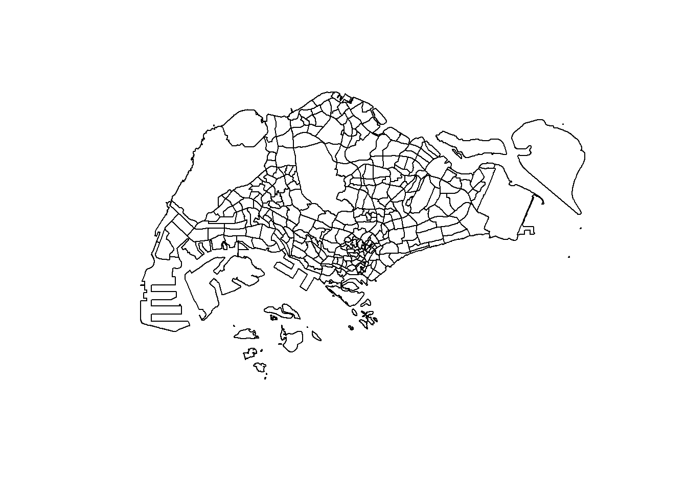
tmap_mode("view")
tm_shape(mrt_sf) +
tm_dots(col="red", size=0.05)tmap_mode("view")
tm_shape(hawker_sf) +
tm_dots(alpha=0.5, #affects transparency of points
col="#d62828",
size=0.05) +
tm_shape(parks_sf) +
tm_dots(alpha=0.5,
col="#f77f00",
size=0.05) +
tm_shape(super_sf) +
tm_dots(alpha=0.5,
col="#fcbf49",
size=0.05) +
tm_shape(mall_sf) +
tm_dots(alpha=0.5,
col="#eae2b7",
size=0.05)Geospatial data wrangling
resale[rowSums(is.na(resale))!=0,]# A tibble: 0 × 11
# … with 11 variables: month <chr>, town <chr>, flat_type <chr>, block <chr>,
# street_name <chr>, storey_range <chr>, floor_area_sqm <dbl>,
# flat_model <chr>, lease_commence_date <dbl>, remaining_lease <chr>,
# resale_price <dbl>length(which(st_is_valid(mpsz_sf) == FALSE))[1] 0Geocoding resale dataframe
This function will geocode the resale dataset by using one map sg API.
library(httr)
geocode <- function(block, streetname) {
base_url <- "https://developers.onemap.sg/commonapi/search"
address <- paste(block, streetname, sep = " ")
query <- list("searchVal" = address,
"returnGeom" = "Y",
"getAddrDetails" = "N",
"pageNum" = "1")
res <- GET(base_url, query = query)
restext<-content(res, as="text")
output <- fromJSON(restext) %>%
as.data.frame %>%
select(results.LATITUDE, results.LONGITUDE)
return(output)
}This takes a really long time to run
# resale$LATITUDE <- 0
#resale$LONGITUDE <- 0
# for (i in 1:nrow(resale)){
# temp_output <- geocode(resale[i, 4], resale[i, 5])
# resale$LATITUDE[i] <- temp_output$results.LATITUDE
# resale$LONGITUDE[i] <- temp_output$results.LONGITUDE
# }#write_rds(resale, "data/model/resale.rds")resale <- read_rds("data/model/resale.rds")unique(resale$storey_range) [1] "01 TO 03" "13 TO 15" "16 TO 18" "07 TO 09" "22 TO 24" "04 TO 06"
[7] "19 TO 21" "10 TO 12" "25 TO 27" "28 TO 30" "34 TO 36" "31 TO 33"
[13] "37 TO 39" "40 TO 42" "43 TO 45" "46 TO 48" "49 TO 51"str_list <- str_split(resale$remaining_lease, " ")
for (i in 1:length(str_list)) {
if (length(unlist(str_list[i])) > 2) {
year <- as.numeric(unlist(str_list[i])[1])
month <- as.numeric(unlist(str_list[i])[3])
resale$remaining_lease[i] <- year + round(month/12, 2)
}
else {
year <- as.numeric(unlist(str_list[i])[1])
resale$remaining_lease[i] <- year
}
}Determining CBD area
lat <- 1.287953
lng <- 103.851784
cbd_sf <- data.frame(lat, lng) %>%
st_as_sf(coords = c("lng", "lat"), crs=4326) %>%
st_transform(crs=3414)sum(is.na(resale$LATITUDE))[1] 0sum(is.na(resale$LONGITUDE))[1] 0resale_sf <- st_as_sf(resale,
coords = c("LONGITUDE",
"LATITUDE"),
# the geographical features are in longitude & latitude, in decimals
# as such, WGS84 is the most appropriate coordinates system
crs=4326) %>%
#afterwards, we transform it to SVY21, our desired CRS
st_transform(crs = 3414)Converting remaining lease from character to numeric
#turning remaining lease from character to numeric
resale_sf$remaining_lease <- as.numeric(as.character(resale_sf$remaining_lease))Turning all unique storey ranges to a numeric value
storeys <- sort(unique(resale_sf$storey_range))storey_order <- 1:length(storeys)
storey_range_order <- data.frame(storeys, storey_order)resale_sf <- left_join(resale_sf, storey_range_order, by= c("storey_range" = "storeys"))Add in the age of unit into the dataset.
age of unit = current year (as of the data) - lease commence date
resale_sf <- resale_sf %>%
add_column(age_of_unit = NA) %>%
mutate(age_of_unit = (
as.numeric(substr(resale_sf$month, 1, 4)) -
as.numeric(resale_sf$lease_commence_date)))Adding in proximity and frequency
proximity <- function(df1, df2, varname) {
dist_matrix <- st_distance(df1, df2) %>%
drop_units()
df1[,varname] <- rowMins(dist_matrix)
return(df1)
}resale_sf <-
proximity(resale_sf, cbd_sf, "PROX_CBD") %>%
proximity(., child_sf, "PROX_CHILDCARE") %>%
proximity(., elder_sf, "PROX_ELDERCARE") %>%
proximity(., hawker_sf, "PROX_HAWKER") %>%
proximity(., mrt_sf, "PROX_MRT") %>%
proximity(., parks_sf, "PROX_PARK") %>%
proximity(., mall_sf, "PROX_MALL") %>%
proximity(., super_sf, "PROX_SPRMKT") %>%
proximity(., prisch_sf, "PROX_TOPPRISCH")num_radius <- function(df1, df2, varname, radius) {
dist_matrix <- st_distance(df1, df2) %>%
drop_units() %>%
as.data.frame()
df1[,varname] <- rowSums(dist_matrix <= radius)
return(df1)
}resale_sf <-
num_radius(resale_sf, kinder_sf, "NUM_KNDRGTN", 350) %>%
num_radius(., child_sf, "NUM_CHILDCARE", 350) %>%
num_radius(., bustop_sf, "NUM_BUS_STOP", 350) %>%
num_radius(., prsc_sf, "NUM_PRI_SCH", 1000)write_rds(resale_sf, "data/model/resale_sf.rds")Exploratory Data Analysis
read_rds("data/model/resale_sf.rds")Simple feature collection with 14519 features and 26 fields
Geometry type: POINT
Dimension: XY
Bounding box: xmin: 6958.193 ymin: 28157.26 xmax: 42645.18 ymax: 48741.06
Projected CRS: SVY21 / Singapore TM
# A tibble: 14,519 × 27
month town flat_…¹ block stree…² store…³ floor…⁴ flat_…⁵ lease…⁶ remai…⁷
<chr> <chr> <chr> <chr> <chr> <chr> <dbl> <chr> <dbl> <dbl>
1 2021-01 ANG MO… 5 ROOM 551 ANG MO… 01 TO … 118 Improv… 1981 59.1
2 2021-01 ANG MO… 5 ROOM 305 ANG MO… 13 TO … 123 Standa… 1977 55.6
3 2021-01 ANG MO… 5 ROOM 520 ANG MO… 16 TO … 118 Improv… 1980 58.7
4 2021-01 ANG MO… 5 ROOM 253 ANG MO… 07 TO … 128 Improv… 1996 74.2
5 2021-01 ANG MO… 5 ROOM 423 ANG MO… 01 TO … 133 Improv… 1993 71.2
6 2021-01 ANG MO… 5 ROOM 617 ANG MO… 13 TO … 133 Model A 1996 74.5
7 2021-01 ANG MO… 5 ROOM 315A ANG MO… 22 TO … 110 Improv… 2006 84.3
8 2021-01 ANG MO… 5 ROOM 596C ANG MO… 13 TO … 110 Improv… 2002 80.9
9 2021-01 ANG MO… 5 ROOM 309A ANG MO… 16 TO … 110 Improv… 2006 84.3
10 2021-01 ANG MO… 5 ROOM 588C ANG MO… 16 TO … 112 DBSS 2011 89.6
# … with 14,509 more rows, 17 more variables: resale_price <dbl>,
# geometry <POINT [m]>, storey_order <int>, age_of_unit <dbl>,
# PROX_CBD <dbl>, PROX_CHILDCARE <dbl>, PROX_ELDERCARE <dbl>,
# PROX_HAWKER <dbl>, PROX_MRT <dbl>, PROX_PARK <dbl>, PROX_MALL <dbl>,
# PROX_SPRMKT <dbl>, PROX_TOPPRISCH <dbl>, NUM_KNDRGTN <dbl>,
# NUM_CHILDCARE <dbl>, NUM_BUS_STOP <dbl>, NUM_PRI_SCH <dbl>, and abbreviated
# variable names ¹flat_type, ²street_name, ³storey_range, ⁴floor_area_sqm, …glimpse(resale_sf)Rows: 14,519
Columns: 27
$ month <chr> "2021-01", "2021-01", "2021-01", "2021-01", "2021-…
$ town <chr> "ANG MO KIO", "ANG MO KIO", "ANG MO KIO", "ANG MO …
$ flat_type <chr> "5 ROOM", "5 ROOM", "5 ROOM", "5 ROOM", "5 ROOM", …
$ block <chr> "551", "305", "520", "253", "423", "617", "315A", …
$ street_name <chr> "ANG MO KIO AVE 10", "ANG MO KIO AVE 1", "ANG MO K…
$ storey_range <chr> "01 TO 03", "13 TO 15", "16 TO 18", "07 TO 09", "0…
$ floor_area_sqm <dbl> 118, 123, 118, 128, 133, 133, 110, 110, 110, 112, …
$ flat_model <chr> "Improved", "Standard", "Improved", "Improved", "I…
$ lease_commence_date <dbl> 1981, 1977, 1980, 1996, 1993, 1996, 2006, 2002, 20…
$ remaining_lease <dbl> 59.08, 55.58, 58.67, 74.25, 71.25, 74.50, 84.33, 8…
$ resale_price <dbl> 483000, 590000, 629000, 670000, 680000, 760000, 76…
$ geometry <POINT [m]> POINT (30820.82 39547.58), POINT (29412.84 3…
$ storey_order <int> 1, 5, 6, 3, 1, 5, 8, 5, 6, 6, 5, 5, 8, 2, 2, 3, 1,…
$ age_of_unit <dbl> 40, 44, 41, 25, 28, 25, 15, 19, 15, 10, 10, 10, 10…
$ PROX_CBD <dbl> 9537.543, 8663.223, 9449.166, 9211.988, 8935.289, …
$ PROX_CHILDCARE <dbl> 2.395193e+02, 1.113894e+02, 1.275906e+02, 1.028995…
$ PROX_ELDERCARE <dbl> 1064.6617, 190.8834, 789.1907, 147.6040, 441.8627,…
$ PROX_HAWKER <dbl> 482.8156, 331.7637, 379.2242, 588.4497, 512.9672, …
$ PROX_MRT <dbl> 1080.8607, 524.3923, 415.9309, 242.7019, 218.2532,…
$ PROX_PARK <dbl> 735.9373, 580.8933, 308.7999, 283.8337, 257.6041, …
$ PROX_MALL <dbl> 1213.2871, 441.6229, 549.4572, 1536.9839, 371.1503…
$ PROX_SPRMKT <dbl> 419.91387, 245.54343, 318.05791, 313.57577, 379.11…
$ PROX_TOPPRISCH <dbl> 274.8829, 1163.7853, 743.7382, 635.2942, 1009.6461…
$ NUM_KNDRGTN <dbl> 1, 1, 1, 1, 1, 1, 1, 0, 1, 1, 1, 1, 1, 1, 0, 0, 1,…
$ NUM_CHILDCARE <dbl> 2, 5, 3, 3, 2, 3, 5, 2, 5, 4, 5, 4, 4, 3, 2, 4, 3,…
$ NUM_BUS_STOP <dbl> 2, 8, 6, 11, 6, 8, 4, 9, 5, 9, 7, 9, 9, 11, 5, 6, …
$ NUM_PRI_SCH <dbl> 3, 3, 5, 2, 4, 4, 3, 5, 2, 4, 4, 4, 4, 4, 3, 3, 3,…summary(resale_sf$resale_price) Min. 1st Qu. Median Mean 3rd Qu. Max.
350000 528000 595000 627297 690000 1418000 graph
ggplot(data=resale_sf, aes(x=resale_price)) +
geom_histogram(bins=20, color="black", fill="light blue") +
labs(title = "Distribution of Resale Prices",
x = "Resale Prices",
y = 'Frequency')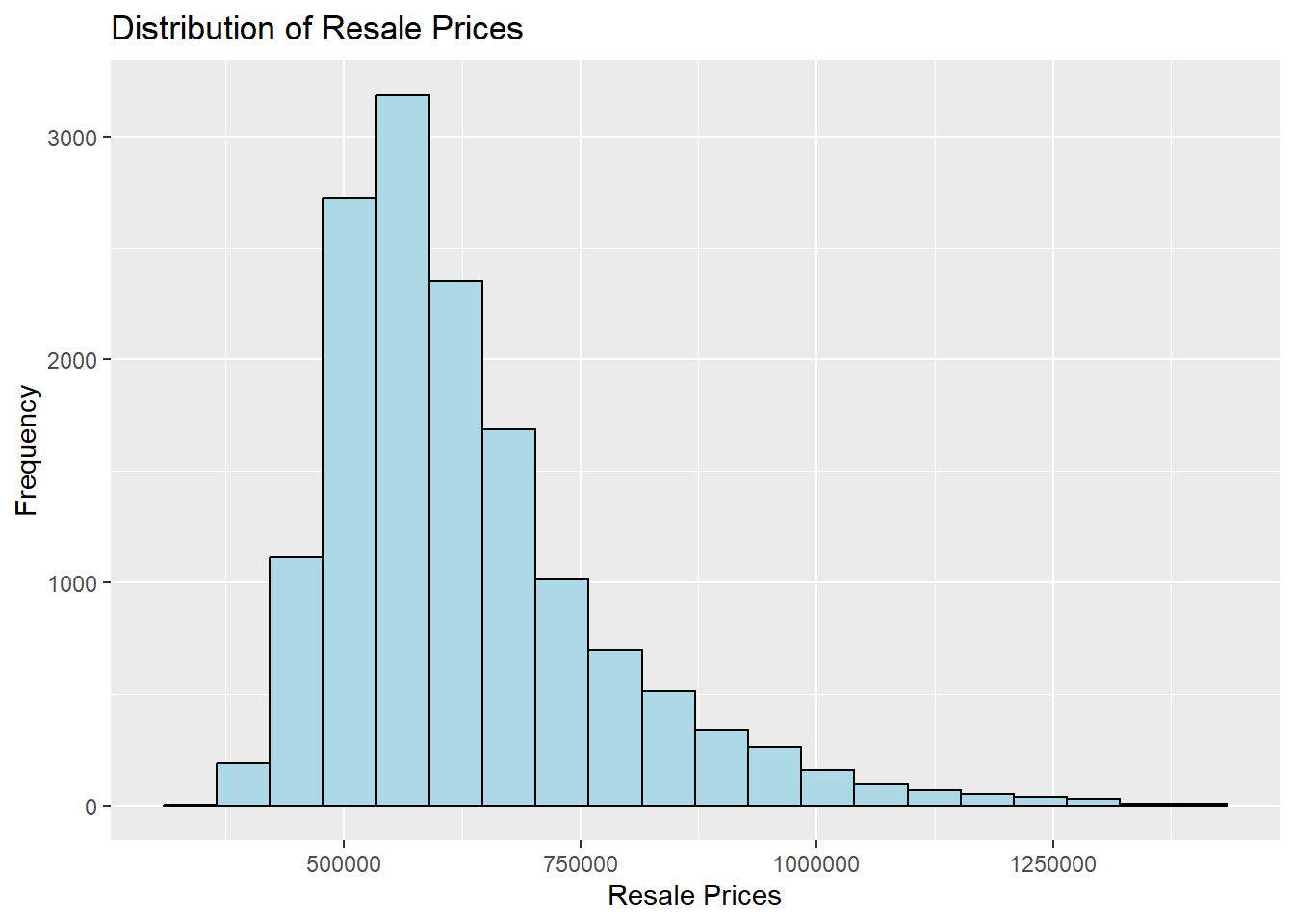
Box plot
ggplot(data = resale_sf, aes(x = '', y = resale_price)) +
geom_boxplot() +
labs(x='', y='Resale Prices')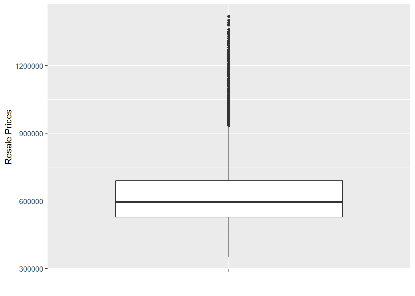
point map
tmap_mode("view")
tmap_options(check.and.fix = TRUE)
tm_shape(resale_sf) +
tm_dots(col = "resale_price",
alpha = 0.6,
style="quantile") +
# sets minimum zoom level to 11, sets maximum zoom level to 14
tm_view(set.zoom.limits = c(11,14))From the plotting of the reslae prices on the map of Singapore, we see that the hdb units in and around central areas of singapore are darker red indicating that they are of higher price. The units in the Western and Northern areas of Singapore are cheaper than those in the Eastern part.
tmap_mode("plot")Top 10 records in terms of price
town_mean <- aggregate(resale_sf[,"resale_price"], list(resale_sf$town), mean)
top10_town = top_n(town_mean, 10, `resale_price`) %>%
arrange(desc(`resale_price`))
top10_townSimple feature collection with 10 features and 2 fields
Geometry type: MULTIPOINT
Dimension: XY
Bounding box: xmin: 6958.193 ymin: 28157.26 xmax: 37492.71 ymax: 38377.45
Projected CRS: SVY21 / Singapore TM
Group.1 resale_price geometry
1 CENTRAL AREA 1054103.5 MULTIPOINT ((28851.09 28922...
2 QUEENSTOWN 915809.2 MULTIPOINT ((22213.08 31972...
3 BUKIT TIMAH 875349.2 MULTIPOINT ((21224.71 35657...
4 BISHAN 840447.2 MULTIPOINT ((27619.38 37901...
5 BUKIT MERAH 833586.2 MULTIPOINT ((25055.59 29894...
6 TOA PAYOH 832569.3 MULTIPOINT ((28957.02 34764...
7 MARINE PARADE 825244.3 MULTIPOINT ((6958.193 32934...
8 CLEMENTI 800793.5 MULTIPOINT ((19953.58 32606...
9 KALLANG/WHAMPOA 799784.5 MULTIPOINT ((22917.56 35326...
10 GEYLANG 748587.1 MULTIPOINT ((32760.87 33216...AREA_SQM <- ggplot(data = resale_sf, aes(x = `floor_area_sqm`)) +
geom_histogram(bins=20, color="black", fill = 'lightblue')
AGE_UNIT <- ggplot(data = resale_sf, aes(x = `age_of_unit`)) +
geom_histogram(bins=20, color="black", fill = 'lightblue')
LEASE_YRS <- ggplot(data = resale_sf, aes(x = `remaining_lease`)) +
geom_histogram(bins=20, color="black", fill = 'lightblue')
PROX_CBD <- ggplot(data = resale_sf, aes(x = `PROX_CBD`)) +
geom_histogram(bins=20, color="black", fill = 'lightblue')
PROX_CHILDCARE <- ggplot(data = resale_sf, aes(x = `PROX_CHILDCARE`)) +
geom_histogram(bins=20, color="black", fill = 'lightblue')
PROX_ELDERCARE <- ggplot(data = resale_sf, aes(x = `PROX_ELDERCARE`)) +
geom_histogram(bins=20, color="black", fill = 'lightblue')
PROX_HAWKER <- ggplot(data = resale_sf, aes(x = `PROX_HAWKER`)) +
geom_histogram(bins=20, color="black", fill = 'lightblue')
PROX_MRT <- ggplot(data = resale_sf, aes(x = `PROX_MRT`)) +
geom_histogram(bins=20, color="black", fill = 'lightblue')
PROX_PARK <- ggplot(data = resale_sf, aes(x = `PROX_PARK`)) +
geom_histogram(bins=20, color="black", fill = 'lightblue')
PROX_TOPPRISCH <- ggplot(data = resale_sf, aes(x = `PROX_TOPPRISCH`)) +
geom_histogram(bins=20, color="black", fill = 'lightblue')
PROX_MALL <- ggplot(data = resale_sf, aes(x = `PROX_MALL`)) +
geom_histogram(bins=20, color="black", fill = 'lightblue')
PROX_SPRMKT <- ggplot(data = resale_sf, aes(x = `PROX_SPRMKT`)) +
geom_histogram(bins=20, color="black", fill = 'lightblue')ggarrange(AREA_SQM, AGE_UNIT, LEASE_YRS, PROX_CBD, PROX_CHILDCARE, PROX_ELDERCARE, PROX_HAWKER, PROX_MRT, PROX_PARK, PROX_TOPPRISCH, PROX_MALL, PROX_SPRMKT, ncol = 3, nrow = 4)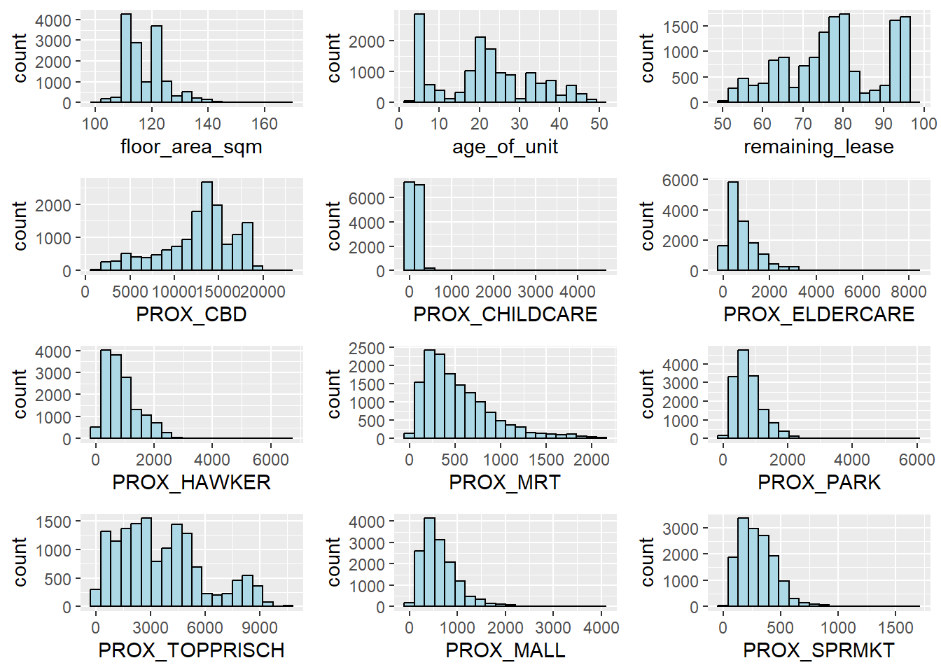
NUM_CHILDCARE <- ggplot(data = resale_sf, aes(x = `NUM_CHILDCARE`)) +
geom_histogram(bins=20, color="black", fill = 'lightblue')
NUM_KNDRGTN <- ggplot(data = resale_sf, aes(x = `NUM_KNDRGTN`)) +
geom_histogram(bins=20, color="black", fill = 'lightblue')
NUM_BUS_STOP <- ggplot(data = resale_sf, aes(x = `NUM_BUS_STOP`)) +
geom_histogram(bins=20, color="black", fill = 'lightblue')
NUM_PRI_SCH <- ggplot(data = resale_sf, aes(x = `NUM_PRI_SCH`)) +
geom_histogram(bins=20, color="black", fill = 'lightblue')
ggarrange(NUM_KNDRGTN, NUM_CHILDCARE, NUM_BUS_STOP, NUM_PRI_SCH, ncol = 2, nrow = 3)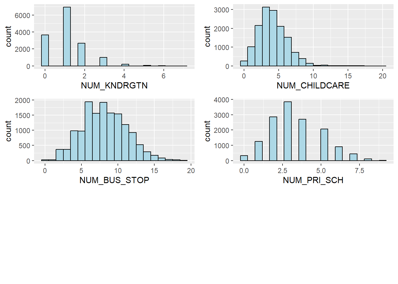
Linear regression
Simple linear regression
resale_slr <- lm(formula=resale_price ~ floor_area_sqm, data = resale_sf)summary(resale_slr)
Call:
lm(formula = resale_price ~ floor_area_sqm, data = resale_sf)
Residuals:
Min 1Q Median 3Q Max
-277295 -99351 -32417 62672 790677
Coefficients:
Estimate Std. Error t value Pr(>|t|)
(Intercept) 6.266e+05 1.953e+04 32.092 <2e-16 ***
floor_area_sqm 5.565e+00 1.660e+02 0.034 0.973
---
Signif. codes: 0 '***' 0.001 '**' 0.01 '*' 0.05 '.' 0.1 ' ' 1
Residual standard error: 146100 on 14517 degrees of freedom
Multiple R-squared: 7.741e-08, Adjusted R-squared: -6.881e-05
F-statistic: 0.001124 on 1 and 14517 DF, p-value: 0.9733ggplot(data=resale_sf,
aes(x=`floor_area_sqm`, y=`resale_price`)) +
geom_point() +
geom_smooth(method = lm)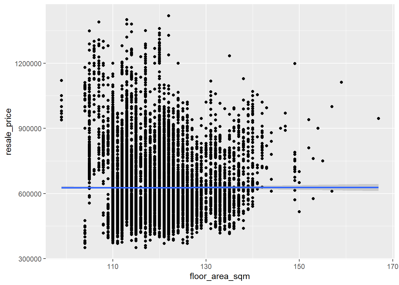
Multiple linear regression
set.seed(1234)
resale_split <- initial_split(resale_sf,
prop = 6.5/10,)
train_data <- training(resale_split)
test_data <- testing(resale_split)#write_rds(train_data, "data/model/train_data.rds")
#write_rds(test_data, "data/model/test_data.rds")Compute correlation matrix
mdata_nogeo <- resale_sf %>%
st_drop_geometry()
corrplot::corrplot(cor(mdata_nogeo[c(7:7, 10:10, 12:26)]),
diag = FALSE,
order = "AOE",
tl.pos = "td",
tl.cex = 0.5,
method = "number",
type = "upper")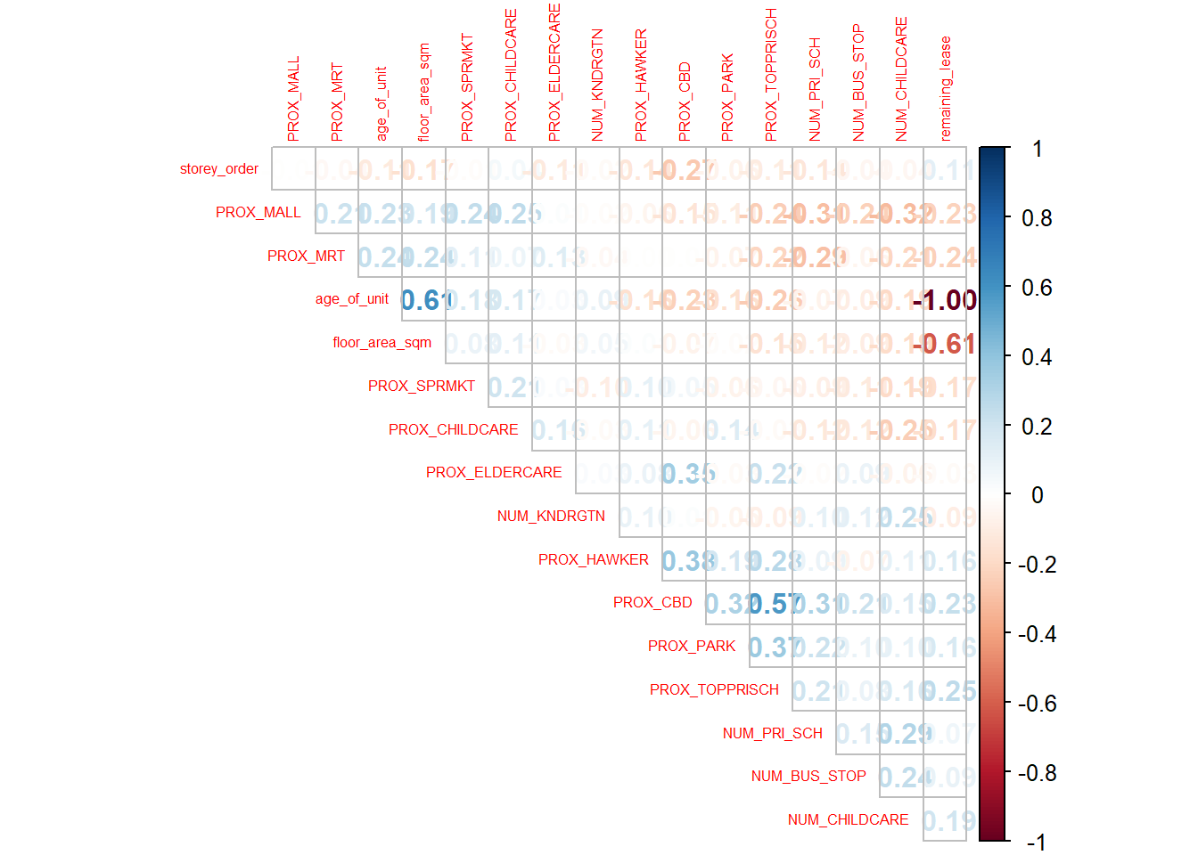
Retrieving stored data
train_data <- read_rds("data/model/train_data.rds")
test_data <- read_rds("data/model/test_data.rds")Building non spatial multiple linear regression
# price_mlr <- lm(resale_price ~ floor_area_sqm + remaining_lease + age_of_unit + storey_order +
# PROX_CBD + PROX_ELDERCARE + PROX_HAWKER +
# PROX_MRT + PROX_PARK + PROX_MALL +
# PROX_SPRMKT + PROX_TOPPRISCH + NUM_KNDRGTN +
# NUM_CHILDCARE + NUM_BUS_STOP +
# NUM_PRI_SCH,
# data=train_data,
# eval = FALSE)
# summary(price_mlr)#write_rds(price_mlr, "data/model/price_mlr.rds" ) price_mlr <-read_rds("data/model/price_mlr.rds")GWR predictive model
train_data_sp <- as_Spatial(train_data)
train_data_spclass : SpatialPointsDataFrame
features : 9437
extent : 6958.193, 42645.18, 28157.26, 48741.06 (xmin, xmax, ymin, ymax)
crs : +proj=tmerc +lat_0=1.36666666666667 +lon_0=103.833333333333 +k=1 +x_0=28001.642 +y_0=38744.572 +ellps=WGS84 +towgs84=0,0,0,0,0,0,0 +units=m +no_defs
variables : 26
names : month, town, flat_type, block, street_name, storey_range, floor_area_sqm, flat_model, lease_commence_date, remaining_lease, resale_price, storey_order, age_of_unit, PROX_CBD, PROX_CHILDCARE, ...
min values : 2021-01, ANG MO KIO, 5 ROOM, 1, ADMIRALTY DR, 01 TO 03, 99, 3Gen, 1972, 49.08, 350000, 1, 2, 1610.9563636452, 0.000104604717071282, ...
max values : 2022-12, YISHUN, 5 ROOM, 9B, ZION RD, 49 TO 51, 167, Type S2, 2019, 96.75, 1418000, 17, 50, 23277.3731998479, 4567.62297445672, ... # bw_adaptive <- bw.gwr(resale_price ~ floor_area_sqm + remaining_lease + age_of_unit+ storey_order +
# PROX_CBD + PROX_ELDERCARE + PROX_HAWKER +
# PROX_MRT + PROX_PARK + PROX_MALL +
# PROX_SPRMKT + PROX_TOPPRISCH + NUM_KNDRGTN +
# NUM_CHILDCARE + NUM_BUS_STOP +
# NUM_PRI_SCH,
# data=train_data_sp,
# approach="CV",
# kernel="gaussian",
# adaptive=TRUE,
# longlat=FALSE,
# eval = FALSE)#write_rds(bw_adaptive, "data/model/bw_adaptive.rds")Constructing adaptive bandwidth gwr model
bw_adaptive <- read_rds("data/model/bw_adaptive.rds")# gwr_adaptive <- gwr.basic(formula = resale_price ~ floor_area_sqm + remaining_lease+ storey_order +
# PROX_CBD + PROX_ELDERCARE + PROX_HAWKER +
# PROX_MRT + PROX_PARK + PROX_MALL +
# PROX_SPRMKT + PROX_TOPPRISCH + NUM_KNDRGTN +
# NUM_CHILDCARE + NUM_BUS_STOP +
# NUM_PRI_SCH,
# data=train_data_sp,
# bw=bw_adaptive,
# kernel = 'gaussian',
# adaptive=TRUE,
# longlat = FALSE,
# eval = FALSE)#write_rds(gwr_adaptive, "data/model/gwr_adaptive.rds")gwr_adaptive <- read_rds("data/model/gwr_adaptive.rds")
gwr_adaptive ***********************************************************************
* Package GWmodel *
***********************************************************************
Program starts at: 2023-03-18 00:03:21
Call:
gwr.basic(formula = resale_price ~ floor_area_sqm + remaining_lease +
storey_order + PROX_CBD + PROX_ELDERCARE + PROX_HAWKER +
PROX_MRT + PROX_PARK + PROX_MALL + PROX_SPRMKT + PROX_TOPPRISCH +
NUM_KNDRGTN + NUM_CHILDCARE + NUM_BUS_STOP + NUM_PRI_SCH,
data = train_data_sp, bw = bw_adaptive, kernel = "gaussian",
adaptive = TRUE, longlat = FALSE)
Dependent (y) variable: resale_price
Independent variables: floor_area_sqm remaining_lease storey_order PROX_CBD PROX_ELDERCARE PROX_HAWKER PROX_MRT PROX_PARK PROX_MALL PROX_SPRMKT PROX_TOPPRISCH NUM_KNDRGTN NUM_CHILDCARE NUM_BUS_STOP NUM_PRI_SCH
Number of data points: 9437
***********************************************************************
* Results of Global Regression *
***********************************************************************
Call:
lm(formula = formula, data = data)
Residuals:
Min 1Q Median 3Q Max
-328797 -53744 -2343 48503 692491
Coefficients:
Estimate Std. Error t value Pr(>|t|)
(Intercept) -1.986e+05 2.446e+04 -8.121 5.21e-16 ***
floor_area_sqm 5.792e+03 1.559e+02 37.155 < 2e-16 ***
remaining_lease 5.582e+03 1.012e+02 55.155 < 2e-16 ***
storey_order 2.019e+04 4.389e+02 46.004 < 2e-16 ***
PROX_CBD -2.001e+01 3.178e-01 -62.966 < 2e-16 ***
PROX_ELDERCARE 2.916e+00 1.483e+00 1.967 0.049264 *
PROX_HAWKER -3.258e+01 1.713e+00 -19.016 < 2e-16 ***
PROX_MRT -2.266e+01 2.572e+00 -8.807 < 2e-16 ***
PROX_PARK 8.416e+00 2.220e+00 3.791 0.000151 ***
PROX_MALL -2.414e+01 2.604e+00 -9.268 < 2e-16 ***
PROX_SPRMKT -5.933e+00 5.775e+00 -1.027 0.304256
PROX_TOPPRISCH -1.417e+00 4.976e-01 -2.848 0.004416 **
NUM_KNDRGTN 4.285e+03 9.738e+02 4.400 1.10e-05 ***
NUM_CHILDCARE -3.200e+03 4.833e+02 -6.622 3.73e-11 ***
NUM_BUS_STOP 2.890e+02 3.079e+02 0.939 0.348011
NUM_PRI_SCH -1.303e+04 6.385e+02 -20.406 < 2e-16 ***
---Significance stars
Signif. codes: 0 '***' 0.001 '**' 0.01 '*' 0.05 '.' 0.1 ' ' 1
Residual standard error: 83990 on 9421 degrees of freedom
Multiple R-squared: 0.6722
Adjusted R-squared: 0.6717
F-statistic: 1288 on 15 and 9421 DF, p-value: < 2.2e-16
***Extra Diagnostic information
Residual sum of squares: 6.645688e+13
Sigma(hat): 83926.48
AIC: 240800.7
AICc: 240800.8
BIC: 231640.9
***********************************************************************
* Results of Geographically Weighted Regression *
***********************************************************************
*********************Model calibration information*********************
Kernel function: gaussian
Adaptive bandwidth: 46 (number of nearest neighbours)
Regression points: the same locations as observations are used.
Distance metric: Euclidean distance metric is used.
****************Summary of GWR coefficient estimates:******************
Min. 1st Qu. Median 3rd Qu. Max.
Intercept -5.7818e+08 -9.0215e+05 2.7616e+04 2.5420e+06 3.2336e+08
floor_area_sqm -4.0891e+05 1.2117e+03 3.4038e+03 5.6121e+03 6.5430e+04
remaining_lease -7.1227e+04 -1.0675e+03 4.2567e+03 6.4094e+03 1.2678e+04
storey_order 1.0768e+03 1.1865e+04 1.4526e+04 1.7808e+04 3.0065e+04
PROX_CBD -3.2747e+04 -1.6686e+02 -2.3985e+01 8.6541e+01 6.6518e+04
PROX_ELDERCARE -2.3479e+04 -4.6628e+01 3.3732e+01 1.3046e+02 5.1293e+03
PROX_HAWKER -1.6979e+04 -7.4513e+01 2.9321e+00 1.1548e+02 5.4425e+04
PROX_MRT -5.7199e+03 -1.1019e+02 -3.7220e+01 5.8608e+01 5.5159e+04
PROX_PARK -4.8577e+04 -1.1170e+02 -1.5924e+01 5.4928e+01 1.0037e+04
PROX_MALL -9.3580e+04 -1.0764e+02 -2.8123e+01 4.7222e+01 1.3162e+04
PROX_SPRMKT -3.2787e+03 -9.7985e+01 -1.8585e+01 6.2931e+01 2.3654e+03
PROX_TOPPRISCH -6.9634e+04 -1.8091e+02 -1.0695e+01 1.9041e+02 3.2801e+04
NUM_KNDRGTN -2.3913e+06 -9.9718e+03 -7.8011e+02 7.7026e+03 9.1610e+04
NUM_CHILDCARE -6.8852e+04 -4.4461e+03 -4.8502e+01 4.7066e+03 1.0285e+05
NUM_BUS_STOP -6.5309e+04 -3.0411e+03 2.4357e+02 3.3927e+03 3.0656e+04
NUM_PRI_SCH -1.1518e+07 -8.6535e+03 -4.2602e+02 8.3385e+03 2.1769e+05
************************Diagnostic information*************************
Number of data points: 9437
Effective number of parameters (2trace(S) - trace(S'S)): 1419.539
Effective degrees of freedom (n-2trace(S) + trace(S'S)): 8017.461
AICc (GWR book, Fotheringham, et al. 2002, p. 61, eq 2.33): 230488.3
AIC (GWR book, Fotheringham, et al. 2002,GWR p. 96, eq. 4.22): 229025.8
BIC (GWR book, Fotheringham, et al. 2002,GWR p. 61, eq. 2.34): 228914.7
Residual sum of squares: 1.696576e+13
R-square value: 0.9163106
Adjusted R-square value: 0.9014911
***********************************************************************
Program stops at: 2023-03-18 00:05:48 coords <- st_coordinates(resale_sf)
coords_train <- st_coordinates(train_data)
coords_test <- st_coordinates(test_data)train_data <- train_data %>%
st_drop_geometry()Calibrating random forest model
# set.seed(1234)
# rf <- ranger(resale_price ~ floor_area_sqm + remaining_lease+ storey_order +
# PROX_CBD + PROX_ELDERCARE + PROX_HAWKER +
# PROX_MRT + PROX_PARK + PROX_MALL +
# PROX_SPRMKT + PROX_TOPPRISCH + NUM_KNDRGTN +
# NUM_CHILDCARE + NUM_BUS_STOP +
# NUM_PRI_SCH,
# data=train_data)#write_rds(rf, "data/model/rf.rds")rf <- read_rds("data/model/rf.rds")print(rf)Ranger result
Call:
ranger(resale_price ~ floor_area_sqm + remaining_lease + storey_order + PROX_CBD + PROX_ELDERCARE + PROX_HAWKER + PROX_MRT + PROX_PARK + PROX_MALL + PROX_SPRMKT + PROX_TOPPRISCH + NUM_KNDRGTN + NUM_CHILDCARE + NUM_BUS_STOP + NUM_PRI_SCH, data = train_data)
Type: Regression
Number of trees: 500
Sample size: 9437
Number of independent variables: 15
Mtry: 3
Target node size: 5
Variable importance mode: none
Splitrule: variance
OOB prediction error (MSE): 2060441912
R squared (OOB): 0.9040941 Calibrating geographically random forest model
Calibrating using training data
# set.seed(1234)
# gwRF_adaptive <- grf(formula = resale_price ~ floor_area_sqm + remaining_lease+ storey_order +
# PROX_CBD + PROX_ELDERCARE + PROX_HAWKER +
# PROX_MRT + PROX_PARK + PROX_MALL +
# PROX_SPRMKT + PROX_TOPPRISCH + NUM_KNDRGTN +
# NUM_CHILDCARE + NUM_BUS_STOP +
# NUM_PRI_SCH,
# dframe=train_data,
# bw=500,
# ntree = 20,
# kernel="adaptive",
# coords=coords_train,
# verbose = T)#write_rds(gwRF_adaptive, "data/model/gwRF_adaptive.rds")gwRF_adaptive <- read_rds("data/model/gwRF_adaptive.rds")Predicting using test data
Predicting GWRF
test_data <- cbind(test_data, coords_test) %>%
st_drop_geometry()# gwRF_pred <- predict.grf(gwRF_adaptive,
# test_data,
# x.var.name="X",
# y.var.name="Y",
# local.w=1,
# global.w=0)# GRF_pred <- write_rds(gwRF_pred, "data/model/GRF_pred.rds")Predicting OLS
mlr_pred <- predict.lm(price_mlr,
test_data,
x.var.name="X",
y.var.name="Y",
local.w=1,
global.w=0)mlr_pred <- write_rds(mlr_pred, "data/model/mlr_pred.rds")Predicting RF
rf_pred <- predict(rf,test_data)rf_pred <- write_rds(rf_pred, "data/model/rf_pred.rds")Converting the predicting output into data frame
Creating GWRF prediction dataframe
GRF_pred <- read_rds("data/model/GRF_pred.rds")
GRF_pred_df <- as.data.frame(GRF_pred)Creating mlr prediction dataframe
mlr_pred <- read_rds("data/model/mlr_pred.rds")
mlr_pred_df <- as.data.frame(mlr_pred)Creating RF prediction dataframe
rf_pred <- read_rds("data/model/rf_pred.rds")
rf_pred_df <- as.data.frame(rf_pred)test_data_p <- cbind(test_data, GRF_pred_df)test_data_mlr <- cbind(test_data, mlr_pred)test_data_rf <- cbind(test_data, rf_pred)#write_rds(test_data_p, "data/model/test_data_p.rds")Calculating RMSE
mlr_pred_df <- read_rds("data/model/mlr_pred.rds") %>%
as.data.frame()
colnames(mlr_pred_df) <- c("mlr_pred")
rf_pred_df <- read_rds("data/model/rf_pred.rds")$predictions %>%
as.data.frame()
colnames(rf_pred_df) <- c("rf_pred")
gwRF_pred_df <- read_rds("data/model/grf_pred.rds") %>%
as.data.frame()
colnames(gwRF_pred_df) <- c("gwrf_pred")
prices_pred_df <- cbind(test_data$resale_price, mlr_pred_df, rf_pred_df,
gwRF_pred_df) %>%
rename("actual_price" = "test_data$resale_price")
head(prices_pred_df) actual_price mlr_pred rf_pred gwrf_pred
1 590000 650874.6 643090.1 628070.2
2 629000 619627.5 664420.1 625059.2
3 670000 739813.9 744091.3 781945.0
4 760000 764903.8 753052.8 797629.5
5 768000 808958.1 843679.0 812444.1
6 816800 679545.5 805450.4 796965.5GWRF
sqrt(mean((prices_pred_df$actual_price - prices_pred_df$gwrf_pred)^2))[1] 43643.26OLS
sqrt(mean((prices_pred_df$actual_price - prices_pred_df$mlr_pred)^2))[1] 83904.36RF
sqrt(mean((prices_pred_df$actual_price - prices_pred_df$rf_pred)^2))[1] 44908.32Through root mean square error calculation we see that RMSE for GWRF prediction has the lowest value, thus showing that this method gives the best predictions of prices. While OLS method has a significantly higher RMSE, showing that it is the most unreliable
Visualizing predicted values
Just to visualize the results of RMSE calculation, lets plot a scatter plot graph
GRF pred
ggplot(data = test_data_p,
aes(x = GRF_pred,
y = resale_price)) +
geom_point()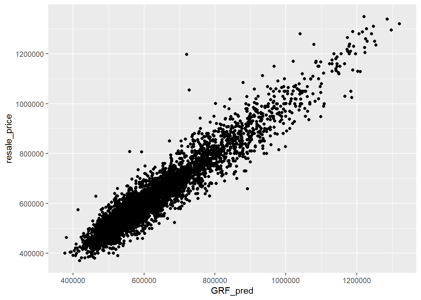
MLR pred
ggplot(data = test_data_mlr,
aes(x = mlr_pred,
y = resale_price)) +
geom_point()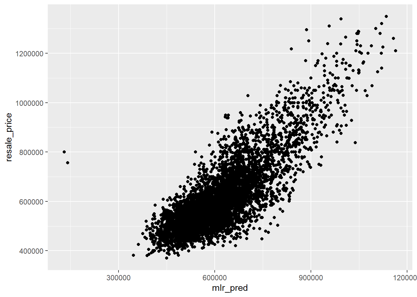
A good predictive model will have the plotted values close to the diagonal line. From our plotting of mlr_pred for OLS, and GRF pred for GWRF we can see that GWRF plotting is closer to the diagonal line. This plot is consistent with our RMSE calculation. hence we can conclude that the geographically weighted random forest method is the best in terms of predicting housing resale prices.