pacman::p_load(sf, tidyverse, tmap, maptools, raster, spatstat, sfdep)Take home assignment 1
Intro
Water is an important resource to mankind. Clean and accessible water is critical to human health. It provides a healthy environment, a sustainable economy, reduces poverty and ensures peace and security. Yet over 40% of the global population does not have access to sufficient clean water. By 2025, 1.8 billion people will be living in countries or regions with absolute water scarcity, according to UN-Water. The lack of water poses a major threat to several sectors, including food security. Agriculture uses about 70% of the world’s accessible freshwater.
Developing countries are most affected by water shortages and poor water quality. Up to 80% of illnesses in the developing world are linked to inadequate water and sanitation. Despite technological advancement, providing clean water to the rural community is still a major development issues in many countries globally, especially countries in the Africa continent.
Objectives
Exploratory Spatial Data Analysis (ESDA)
Derive kernel density maps of functional and non-functional water points. Using appropriate tmap functions
Display the kernel density maps on openstreetmap of Osub State, Nigeria.
Describe the spatial patterns revealed by the kernel density maps. Highlight the advantage of kernel density map over point map.
Second-order Spatial Point Patterns Analysis
With reference to the spatial point patterns observed in ESDA:
Formulate the null hypothesis and alternative hypothesis and select the confidence level.
Perform the test by using appropriate Second order spatial point patterns analysis technique.
With reference to the analysis results, draw statistical conclusions.
Spatial Correlation Analysis
In this section, you are required to confirm statistically if the spatial distribution of functional and non-functional water points are independent from each other.
Formulate the null hypothesis and alternative hypothesis and select the confidence level.
Perform the test by using appropriate Second order spatial point patterns analysis technique.
With reference to the analysis results, draw statistical conclusions.
Importing packages
Data wrangling
Import Aspatial data
First we take the Wpdx dataset and filter out to get only one country data: Nigeria, then filter out to get only one state: Osun
wp_nga <- read_csv("data/aspatial/WPdx.csv") %>%
  filter(`#clean_country_name` == "Nigeria", `#clean_adm1` == "Osun")
Import Geospatial data
geoNGA <- st_read(dsn = "data/geospatial",
                  layer = "geoBoundaries-NGA-ADM2")%>%

  st_transform(crs = 26392)
Reading layer `geoBoundaries-NGA-ADM2' from data source
`C:\Study\Y3\S2\IS415\ELAbishek\IS415-GAA\Takehome_exercise\TakeHome1\data\geospatial'
using driver `ESRI Shapefile'
Simple feature collection with 774 features and 5 fields
Geometry type: MULTIPOLYGON
Dimension: XY
Bounding box: xmin: 2.668534 ymin: 4.273007 xmax: 14.67882 ymax: 13.89442
Geodetic CRS: WGS 84Now we take the geospatial dataset and we filter out to get only the data from Osun state
NGA <- st_read("data/geospatial",
               layer = "nga_admbnda_adm2")%>%
  filter(`ADM1_EN` == "Osun")%>%
  st_transform(crs = 26392)
Reading layer `nga_admbnda_adm2' from data source
`C:\Study\Y3\S2\IS415\ELAbishek\IS415-GAA\Takehome_exercise\TakeHome1\data\geospatial'
using driver `ESRI Shapefile'
Simple feature collection with 774 features and 16 fields
Geometry type: MULTIPOLYGON
Dimension: XY
Bounding box: xmin: 2.668534 ymin: 4.273007 xmax: 14.67882 ymax: 13.89442
Geodetic CRS: WGS 84Data pre processing
Convert Aspatial data into Geospatial
wp_nga$Geometry = st_as_sfc(wp_nga$`New Georeferenced Column`)
glimpse(wp_nga)
Rows: 5,557
Columns: 71
$ row_id <dbl> 429123, 70566, 70578, 66401, 422190, 422…
$ `#source` <chr> "GRID3", "Federal Ministry of Water Reso…
$ `#lat_deg` <dbl> 8.020000, 7.317741, 7.759448, 8.031187, …
$ `#lon_deg` <dbl> 5.060000, 4.785507, 4.563998, 4.637400, …
$ `#report_date` <chr> "08/29/2018 12:00:00 AM", "05/11/2015 12…
$ `#status_id` <chr> "Unknown", "No", "No", "No", "Unknown", …
$ `#water_source_clean` <chr> NA, "Protected Shallow Well", "Borehole"…
$ `#water_source_category` <chr> NA, "Well", "Well", "Well", NA, NA, "Wel…
$ `#water_tech_clean` <chr> "Tapstand", "Mechanized Pump", "Mechaniz…
$ `#water_tech_category` <chr> "Tapstand", "Mechanized Pump", "Mechaniz…
$ `#facility_type` <chr> "Improved", "Improved", "Improved", "Imp…
$ `#clean_country_name` <chr> "Nigeria", "Nigeria", "Nigeria", "Nigeri…
$ `#clean_adm1` <chr> "Osun", "Osun", "Osun", "Osun", "Osun", …
$ `#clean_adm2` <chr> "Ifedayo", "Atakumosa East", "Osogbo", "…
$ `#clean_adm3` <chr> NA, NA, NA, NA, NA, NA, NA, NA, NA, NA, …
$ `#clean_adm4` <chr> NA, NA, NA, NA, NA, NA, NA, NA, NA, NA, …
$ `#install_year` <dbl> NA, NA, NA, 2004, NA, NA, 2006, 2014, 20…
$ `#installer` <chr> NA, NA, NA, NA, NA, NA, NA, NA, NA, NA, …
$ `#rehab_year` <lgl> NA, NA, NA, NA, NA, NA, NA, NA, NA, NA, …
$ `#rehabilitator` <lgl> NA, NA, NA, NA, NA, NA, NA, NA, NA, NA, …
$ `#management_clean` <chr> NA, NA, NA, NA, NA, NA, NA, NA, NA, "Com…
$ `#status_clean` <chr> NA, "Abandoned/Decommissioned", "Abandon…
$ `#pay` <chr> NA, "No", "No", "No", NA, NA, "No", "No"…
$ `#fecal_coliform_presence` <chr> NA, NA, NA, NA, NA, NA, NA, NA, NA, NA, …
$ `#fecal_coliform_value` <dbl> NA, NA, NA, NA, NA, NA, NA, NA, NA, NA, …
$ `#subjective_quality` <chr> NA, "Acceptable quality", "Acceptable qu…
$ `#activity_id` <chr> "6054e946-2573-45bf-ab7c-0ddaa68a61b4", …
$ `#scheme_id` <chr> NA, NA, NA, NA, NA, NA, NA, NA, NA, NA, …
$ `#wpdx_id` <chr> "6FW723C6+222", "6FV68Q9P+36R", "6FV6QH5…
$ `#notes` <chr> "Rt Hon Kola Oluwawole Water Tap", "Temi…
$ `#orig_lnk` <chr> "https://nigeria.africageoportal.com/dat…
$ `#photo_lnk` <chr> NA, "https://akvoflow-55.s3.amazonaws.co…
$ `#country_id` <chr> "NG", "NG", "NG", "NG", "NG", "NG", "NG"…
$ `#data_lnk` <chr> "https://catalog.waterpointdata.org/data…
$ `#distance_to_primary_road` <dbl> 4474.22234, 10130.42742, 167.82235, 4133…
$ `#distance_to_secondary_road` <dbl> 1883.98780, 17466.35720, 838.91849, 1162…
$ `#distance_to_tertiary_road` <dbl> 1885.874322, 2376.832183, 1181.107236, 9…
$ `#distance_to_city` <dbl> 40100.268, 31549.222, 2449.293, 16704.19…
$ `#distance_to_town` <dbl> 8120.871, 24652.907, 9463.295, 5176.899,…
$ water_point_history <chr> "{\"2018-08-29\": {\"source\": \"GRID3\"…
$ rehab_priority <dbl> NA, NA, NA, NA, NA, NA, NA, NA, NA, NA, …
$ water_point_population <dbl> NA, NA, NA, NA, NA, NA, NA, NA, 0, 508, …
$ local_population_1km <dbl> NA, NA, NA, NA, NA, NA, NA, NA, 70, 647,…
$ crucialness_score <dbl> NA, NA, NA, NA, NA, NA, NA, NA, NA, 0.78…
$ pressure_score <dbl> NA, NA, NA, NA, NA, NA, NA, NA, NA, 1.69…
$ usage_capacity <dbl> 250, 1000, 1000, 1000, 250, 250, 1000, 3…
$ is_urban <lgl> FALSE, FALSE, TRUE, FALSE, FALSE, FALSE,…
$ days_since_report <dbl> 1483, 2689, 2689, 2700, 1483, 1483, 2688…
$ staleness_score <dbl> 62.65911, 42.84384, 42.84384, 42.69554, …
$ latest_record <lgl> TRUE, TRUE, TRUE, TRUE, TRUE, TRUE, TRUE…
$ location_id <dbl> 358783, 239555, 239556, 230405, 358062, …
$ cluster_size <dbl> 1, 1, 1, 1, 1, 1, 1, 1, 1, 1, 1, 1, 1, 1…
$ `#clean_country_id` <chr> "NGA", "NGA", "NGA", "NGA", "NGA", "NGA"…
$ `#country_name` <chr> "Nigeria", "Nigeria", "Nigeria", "Nigeri…
$ `#water_source` <chr> "Tap", "Improved Protected dug well", "I…
$ `#water_tech` <chr> NA, "Motorised", "Motorised", "Motorised…
$ `#status` <chr> NA, "Non-functional Abandoned", "Non-fun…
$ `#adm2` <chr> NA, "Atakumosa East", "Osogbo", "Odo-Oti…
$ `#adm3` <chr> NA, NA, NA, NA, NA, NA, NA, NA, NA, NA, …
$ `#management` <chr> NA, NA, NA, NA, NA, NA, NA, NA, NA, "Com…
$ `#adm1` <chr> NA, "Osun", "Osun", "Osun", NA, NA, "Osu…
$ `New Georeferenced Column` <chr> "POINT (5.06 8.02)", "POINT (4.7855068 7…
$ lat_deg_original <dbl> NA, NA, NA, NA, NA, NA, NA, NA, NA, NA, …
$ lat_lon_deg <chr> "(8.02°, 5.06°)", "(7.3177411°, 4.785506…
$ lon_deg_original <dbl> NA, NA, NA, NA, NA, NA, NA, NA, NA, NA, …
$ public_data_source <chr> "https://catalog.waterpointdata.org/data…
$ converted <chr> NA, "#status_id, #water_source, #pay, #s…
$ count <dbl> 1, 1, 1, 1, 1, 1, 1, 1, 1, 1, 1, 1, 1, 1…
$ created_timestamp <chr> "12/06/2021 09:12:57 PM", "06/30/2020 12…
$ updated_timestamp <chr> "12/06/2021 09:12:57 PM", "06/30/2020 12…
$ Geometry <POINT> POINT (5.06 8.02), POINT (4.785507 7.3…wp_sf <- st_sf(wp_nga, crs=4326)
wp_sfSimple feature collection with 5557 features and 70 fields
Geometry type: POINT
Dimension: XY
Bounding box: xmin: 4.032004 ymin: 7.060309 xmax: 5.06 ymax: 8.061898
Geodetic CRS: WGS 84
# A tibble: 5,557 × 71
row_id `#source` #lat_…¹ #lon_…² #repo…³ #stat…⁴ #wate…⁵ #wate…⁶ #wate…⁷
* <dbl> <chr> <dbl> <dbl> <chr> <chr> <chr> <chr> <chr>
1 429123 GRID3 8.02 5.06 08/29/… Unknown <NA> <NA> Tapsta…
2 70566 Federal Minis… 7.32 4.79 05/11/… No Protec… Well Mechan…
3 70578 Federal Minis… 7.76 4.56 05/11/… No Boreho… Well Mechan…
4 66401 Federal Minis… 8.03 4.64 04/30/… No Boreho… Well Mechan…
5 422190 GRID3 7.87 4.88 08/29/… Unknown <NA> <NA> Tapsta…
6 422064 GRID3 7.7 4.89 08/29/… Unknown <NA> <NA> Tapsta…
7 65607 Federal Minis… 7.89 4.71 05/12/… No Boreho… Well Mechan…
8 68989 Federal Minis… 7.51 4.27 05/07/… No Boreho… Well <NA>
9 67708 Federal Minis… 7.48 4.35 04/29/… Yes Boreho… Well Mechan…
10 66419 Federal Minis… 7.63 4.50 05/08/… Yes Boreho… Well Hand P…
# … with 5,547 more rows, 62 more variables: `#water_tech_category` <chr>,
# `#facility_type` <chr>, `#clean_country_name` <chr>, `#clean_adm1` <chr>,
# `#clean_adm2` <chr>, `#clean_adm3` <chr>, `#clean_adm4` <chr>,
# `#install_year` <dbl>, `#installer` <chr>, `#rehab_year` <lgl>,
# `#rehabilitator` <lgl>, `#management_clean` <chr>, `#status_clean` <chr>,
# `#pay` <chr>, `#fecal_coliform_presence` <chr>,
# `#fecal_coliform_value` <dbl>, `#subjective_quality` <chr>, …Projection transformation
We then transform the dataset into appropriate crs = 26392 so that we can perform our further analysis
wp_sf <- wp_sf %>%
  st_transform(crs = 26392)
Selecting necessary columns
There is no need for the other columns, so we are taking just the column we need, just to make things faster in the long run
NGA <- NGA %>%
 dplyr::select(c(3:4, 8:9)) #adm1 and adm2 cols
Cleaning duplicate data
NGA$ADM2_EN[duplicated(NGA$ADM2_EN)==TRUE]character(0)duplicated_LGA <- NGA$ADM2_EN[duplicated(NGA$ADM2_EN)==TRUE]
duplicated_indices <- which(NGA$ADM2_EN %in% duplicated_LGA)
for (ind in duplicated_indices) {
NGA$ADM2_EN[ind] <- paste(NGA$ADM2_EN[ind], NGA$ADM1_EN[ind], sep=", ")
}Now that we have assurance that the data does not have any duplicate data, we may proceed with data wrangling
Data wrangling
#Replacing records where the status column is empty with "unknown" to prevent errors in the future
wp_sf <- wp_sf %>%
  rename(status_clean = '#status_clean') %>%
  dplyr::select(status_clean) %>%
  mutate(status_clean = replace_na(
    status_clean, "unknown"
  ))
wp_sf_osun <- wp_sf %>%
mutate(`func_status` = case_when(
`status_clean` %in% c("Functional",
"Functional but not in use",
"Functional but needs repair") ~
"Functional",
`status_clean` %in% c("Abandoned/Decommissioned",
"Non-Functional due to dry season",
"Non-Functional",
"Abandoned",
"Non functional due to dry season") ~
"Non-Functional",
`status_clean` == "Unknown" ~ "Unknown"))Separating functional and non functional waterpoints
Separating out and obtaining functional and non functional waterpoints
wp_functional <- wp_sf_osun %>%
  filter(status_clean %in%
           c("Functional",
             "Functional but not in use",
             "Functional but needs repair"))
wp_nonfunctional <- wp_sf_osun %>%
filter(status_clean %in%
c("Abandoned/Decommissioned",
"Abandoned",
"Non-Functional due to dry season",
"Non-Functional",
"Non functional due to dry season"))wp_unknown_sf <- wp_sf_osun %>% filter(`status_clean` %in%
c("unknown"))NGA_wp_sf <- NGA %>%
mutate(`total_wp` = lengths(
st_intersects(NGA, wp_sf_osun)
)) %>%
mutate(`wp_functional` = lengths(
st_intersects(NGA, wp_functional)
)) %>%
mutate(`wp_nonfunctional` = lengths(
st_intersects(NGA, wp_nonfunctional)
)) %>%
mutate(`wp_unknown_sf` = lengths(
st_intersects(NGA, wp_unknown_sf)
))glimpse(NGA)Rows: 30
Columns: 5
$ ADM2_EN <chr> "Aiyedade", "Aiyedire", "Atakumosa East", "Atakumosa West",…
$ ADM2_PCODE <chr> "NG030001", "NG030002", "NG030003", "NG030004", "NG030005",…
$ ADM1_EN <chr> "Osun", "Osun", "Osun", "Osun", "Osun", "Osun", "Osun", "Os…
$ ADM1_PCODE <chr> "NG030", "NG030", "NG030", "NG030", "NG030", "NG030", "NG03…
$ geometry <MULTIPOLYGON [m]> MULTIPOLYGON (((213526.6 34..., MULTIPOLYGON (…Kernel Density Estimation
NG <- as_Spatial(NGA)
wpf <- as_Spatial(wp_functional)
wpnf <- as_Spatial(wp_nonfunctional)
Converting to sp
NG_sp <- as(NG, "SpatialPolygons")
wpf_sp <- as(wpf,"SpatialPoints")
wpnf_sp <- as(wpnf, "SpatialPoints")
Creation of owin object
NG_owin <- as(NG_sp, "owin")Converting sp to ppp object
wpf_ppp <- as(wpf_sp, "ppp")
wpnf_ppp <- as(wpnf_sp, "ppp")plot(wpf_ppp)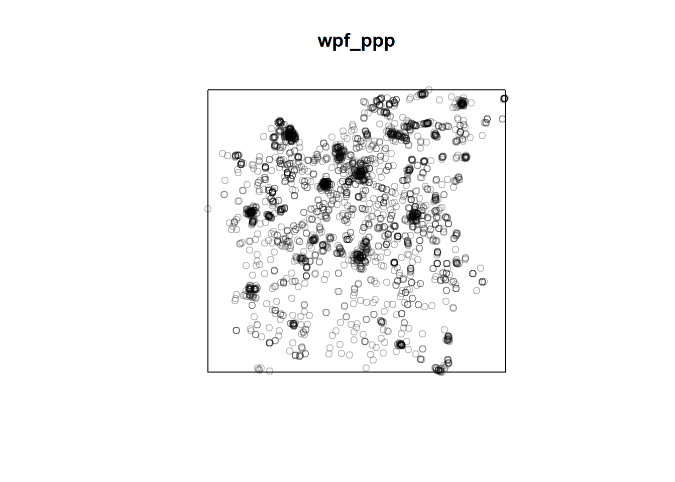
plot(wpnf_ppp)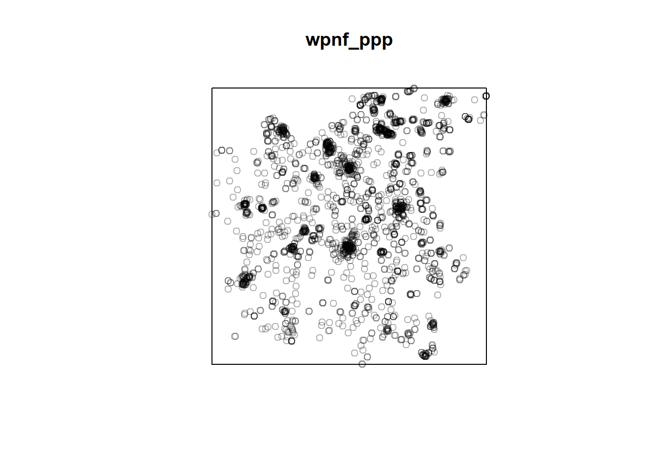
wpf_ppp = wpf_ppp[NG_owin]
wpnf_ppp = wpnf_ppp[NG_owin]plot(wpf_ppp)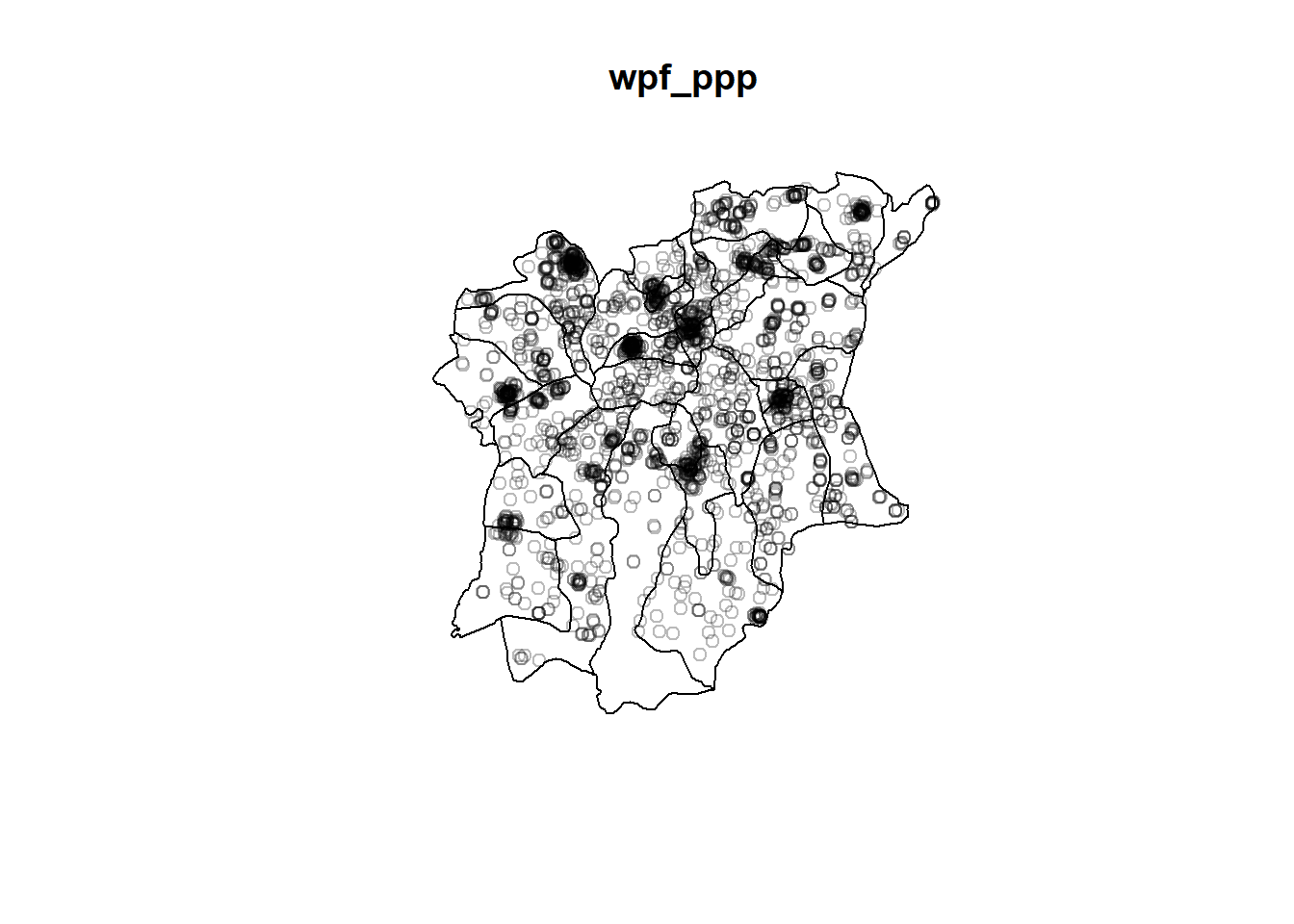
plot(wpnf_ppp)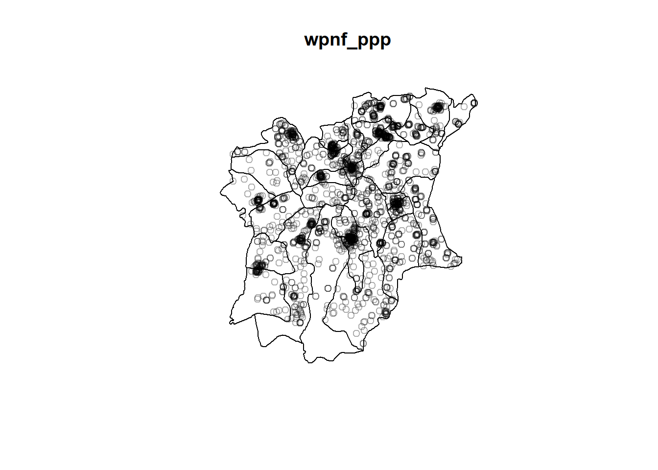
Checking for duplicate values
any(duplicated(wpf_ppp)) [1] FALSEany(duplicated(wpnf_ppp)) [1] FALSESince no duplicate values were detected, we can proceed with the plotting as per normal
NGAf_bw <- density(wpf_ppp,
                              sigma=bw.ppl,
                              edge=TRUE,
                            kernel="gaussian")
NGAnf_bw <- density(wpnf_ppp,
                              sigma=bw.ppl,
                              edge=TRUE,
                            kernel="gaussian")
Scaling of the ppp so that we can get accurate mapping that is consistent
wpf_ppp.km <- rescale(wpf_ppp, 1000, "km")
wpnf_ppp.km <- rescale(wpnf_ppp, 1000, "km")
bw <- bw.ppl(wpf_ppp)
bw sigma
919.2953 bw <- bw.ppl(wpnf_ppp)
bw sigma
973.7385 NGAf.bw <- density(wpf_ppp.km, sigma=bw.ppl, edge=TRUE, kernel="gaussian")
NGAnf.bw <- density(wpnf_ppp.km, sigma=bw.ppl, edge=TRUE, kernel="gaussian")
plot(NGAnf.bw)
plot(NGAf.bw)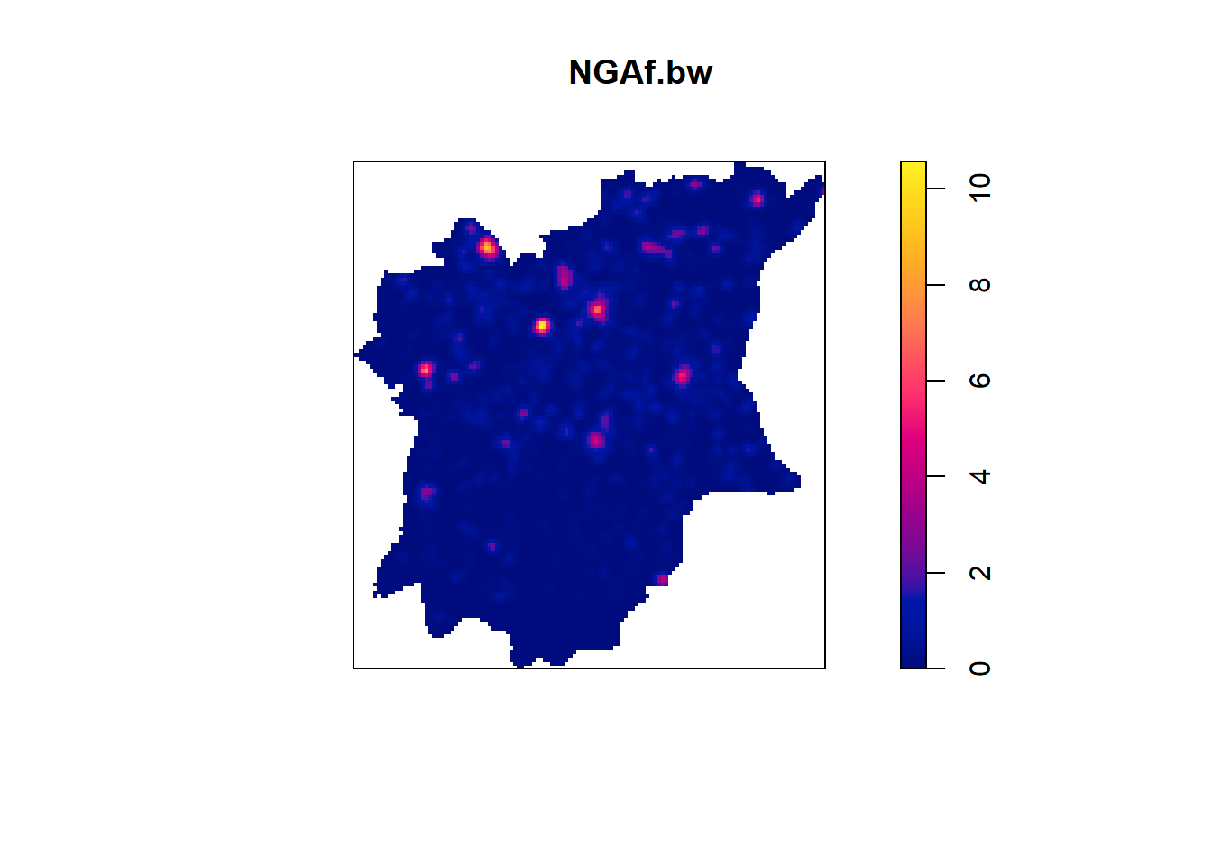
Converting KDE into grid object
gridded_NGAf_bw <- as.SpatialGridDataFrame.im(NGAf.bw)
spplot(gridded_NGAf_bw)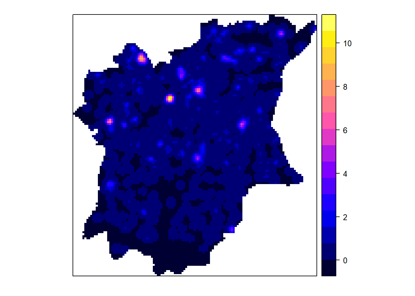
gridded_NGAnf_bw <- as.SpatialGridDataFrame.im(NGAnf.bw)
spplot(gridded_NGAnf_bw)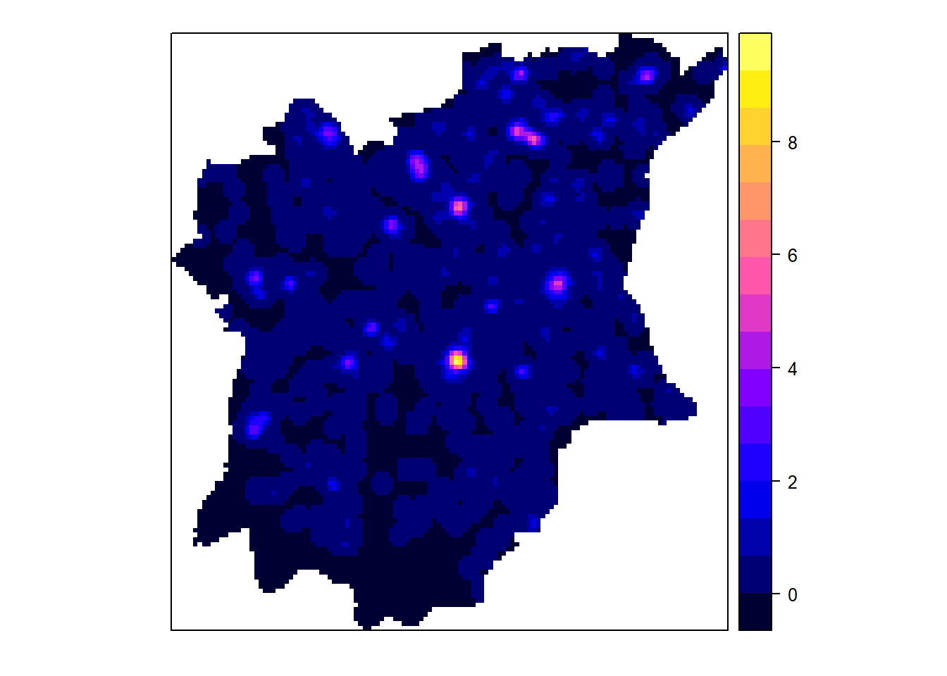
Converting gridded output into raster
NGAf_bw_raster <- raster(gridded_NGAf_bw)

NGAnf_bw_raster <- raster(gridded_NGAnf_bw)NGAf_bw_rasterclass : RasterLayer
dimensions : 128, 128, 16384 (nrow, ncol, ncell)
resolution : 0.8948485, 0.9616045 (x, y)
extent : 176.5032, 291.0438, 331.4347, 454.5201 (xmin, xmax, ymin, ymax)
crs : NA
source : memory
names : v
values : -4.99773e-16, 10.55944 (min, max)NGAnf_bw_rasterclass : RasterLayer
dimensions : 128, 128, 16384 (nrow, ncol, ncell)
resolution : 0.8948485, 0.9616045 (x, y)
extent : 176.5032, 291.0438, 331.4347, 454.5201 (xmin, xmax, ymin, ymax)
crs : NA
source : memory
names : v
values : -2.52505e-16, 9.25861 (min, max)projection(NGAf_bw_raster) <- CRS("+init=EPSG:26392 +units=km")
NGAf_bw_rasterclass : RasterLayer
dimensions : 128, 128, 16384 (nrow, ncol, ncell)
resolution : 0.8948485, 0.9616045 (x, y)
extent : 176.5032, 291.0438, 331.4347, 454.5201 (xmin, xmax, ymin, ymax)
crs : +init=EPSG:26392 +units=km
source : memory
names : v
values : -4.99773e-16, 10.55944 (min, max)projection(NGAnf_bw_raster) <- CRS("+init=EPSG:26392 +units=km")
NGAnf_bw_rasterclass : RasterLayer
dimensions : 128, 128, 16384 (nrow, ncol, ncell)
resolution : 0.8948485, 0.9616045 (x, y)
extent : 176.5032, 291.0438, 331.4347, 454.5201 (xmin, xmax, ymin, ymax)
crs : +init=EPSG:26392 +units=km
source : memory
names : v
values : -2.52505e-16, 9.25861 (min, max)KDE on open street map
Plotting KDE for functional waterpoints
tmap_mode('view')+ #Functional KDE
  tm_shape(NGAf_bw_raster) +
  tm_raster("v", palette = "YlOrBr") +
  tm_basemap("OpenStreetMap") +
  tm_layout(legend.position = c("right", "bottom"), frame = FALSE)
kde_func <- tm_shape(NGAf_bw_raster) +
tm_raster("v", palette = "YlOrBr", title="") +
tm_layout(
legend.position = c("right", "bottom"),
main.title = "Functional",
frame = FALSE
)
kde_func +
tm_shape(NGA) +
tm_borders() +
tm_text("ADM2_EN", size = 0.6) Plotting KDE for non functional waterpoints
tmap_mode('view')+ #Non-functional KDE
  tm_shape(NGAnf_bw_raster) +
  tm_raster("v", alpha = 0.75, palette = "YlGnBu") +
  tm_basemap("OpenStreetMap") +
  tm_layout(legend.position = c("right", "bottom"), frame = FALSE)
kde_nonfunc <- tm_shape(NGAnf_bw_raster) +
tm_raster("v", palette = "YlGnBu", title="") +
tm_layout(
legend.position = c("right", "bottom"),
main.title = "Non-Functional",
frame = FALSE
)
kde_nonfunc +
tm_shape(NGA) +
tm_borders() +
tm_text("ADM2_EN", size = 0.6)Analysis
From the KDE plots done above we can see that there is a huge disparity in terms of the concentration of functional to nonfunctional waterpoints in the different LGAs of Osun state. There is a higher number of water points in the Northern parts of the state, but in that, the North Western LGAs have a higher concentration of Functional waterpoints, such as Ife North, Ejigbo, and Iwo. While the North Easter LGAs have a higher concentration of non functional water points, such as in LGAs like Osogobo, Irepodun, Boripe. Ife Central also has a really high concentration of non functional waterpoints in its Southern section.
Second order spatial point analysis
In order to perform second order spatial point analysis, in this case we are creating owin objects of some LGAs within Osun for observation
H0: Functional and non functional waterpoints are randomly distributed
H1: Functional and non functional waterpoints are not randomly distributed
Confidence level : 99%
Significance level (alpha) : 0.05
Reject null hypothesis if p-value is < 0.05
#Functional water points
IfeCentralowin <- NGA[NGA$ADM2_EN == "Ife Central",] %>%
    as('Spatial') %>%
    as('SpatialPolygons') %>%
    as('owin')

Ejigboowin <- NGA[NGA$ADM2_EN == "Ejigbo",] %>%
    as('Spatial') %>%
    as('SpatialPolygons') %>%
    as('owin')

#non functional points
EdeNorthowin <- NGA[NGA$ADM2_EN == "Ede North",] %>%
    as('Spatial') %>%
    as('SpatialPolygons') %>%
    as('owin')

EdeSouthowin <- NGA[NGA$ADM2_EN == "Ede South",] %>%
    as('Spatial') %>%
    as('SpatialPolygons') %>%
    as('owin')

plot(IfeCentralowin)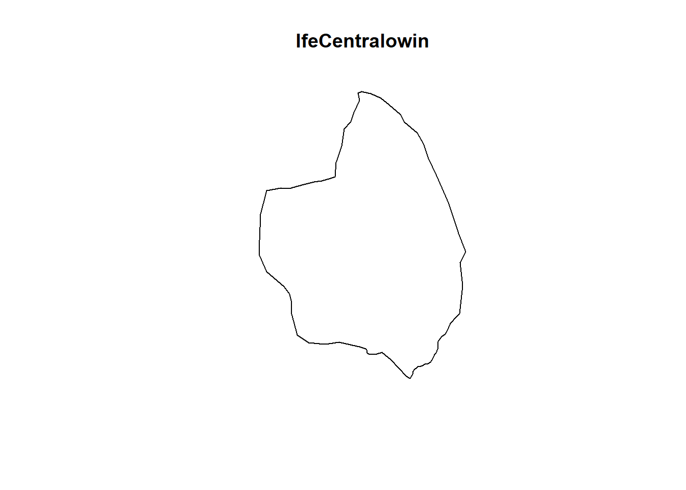
plot(Ejigboowin)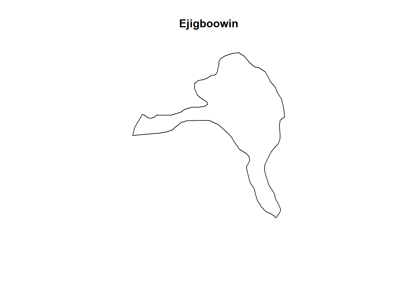
plot(EdeNorthowin)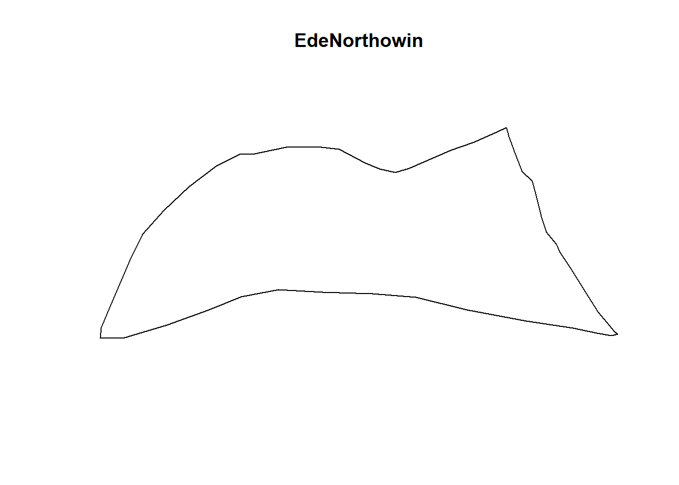
plot(EdeSouthowin)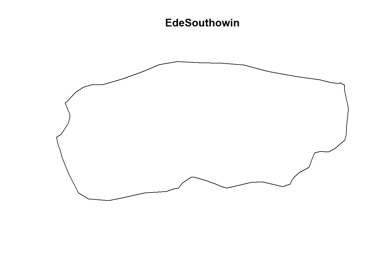
IfeCentralowin_ppp <- wpf_ppp[IfeCentralowin]
Ejigboowin_ppp <- wpf_ppp[Ejigboowin]
EdeNorthowin_ppp <- wpnf_ppp[EdeNorthowin]
EdeSouthowin_ppp <- wpnf_ppp[EdeSouthowin]plot(IfeCentralowin_ppp)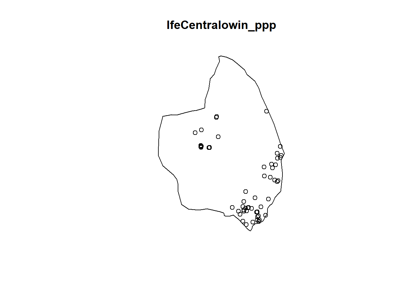
plot(Ejigboowin_ppp)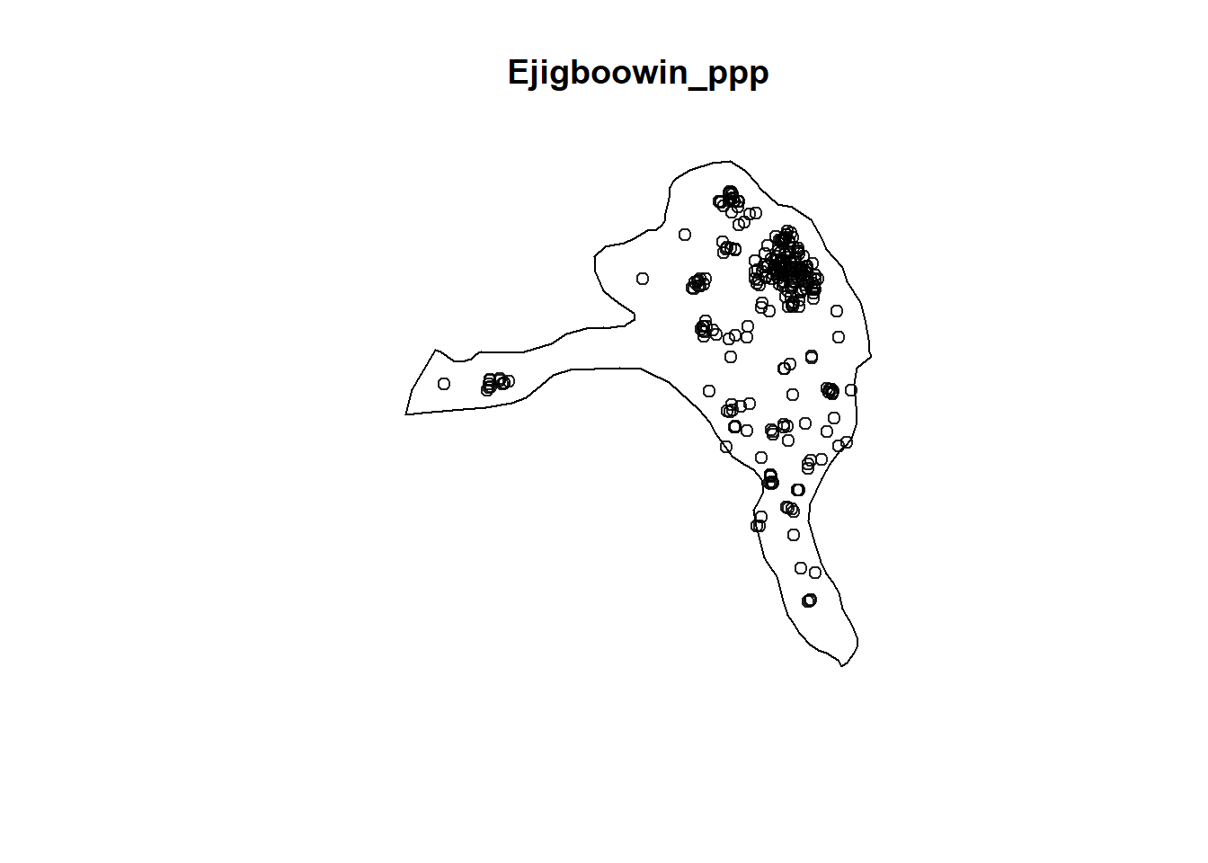
plot(EdeNorthowin_ppp)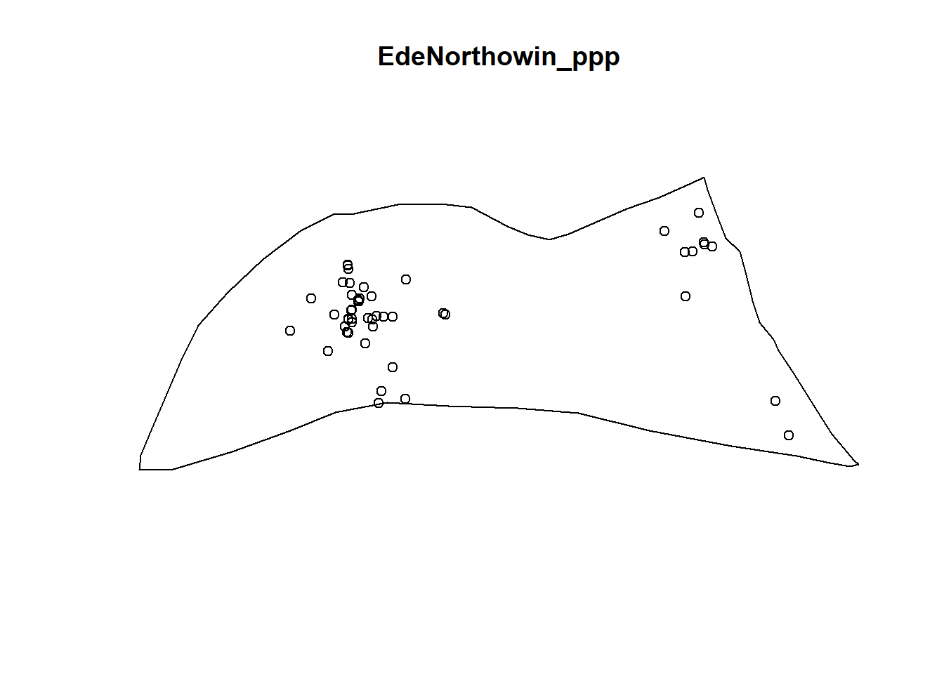
plot(EdeSouthowin_ppp)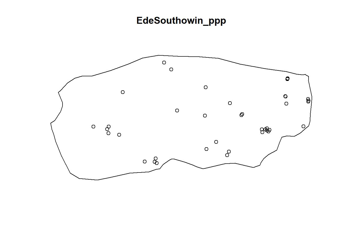
Now that we have the owin objects with the functional and non functional water points plotted in them, we can start off by plotting the G function
Plotting G function for functional waterpoints
IfecentralFuncG = Gest(IfeCentralowin_ppp, correction = "border")
plot(IfecentralFuncG)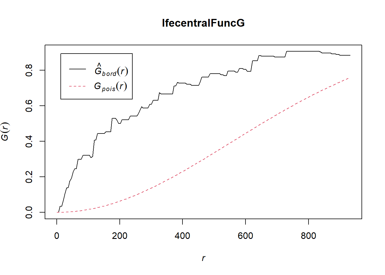
Spatial randomness test
IfecentralFunc.csr <- envelope(IfeCentralowin_ppp, Gest, nsim=100)Generating 100 simulations of CSR ...
1, 2, 3, 4, 5, 6, 7, 8, 9, 10, 11, 12, 13, 14, 15, 16, 17, 18, 19, 20, 21, 22, 23, 24, 25, 26, 27, 28, 29, 30, 31, 32, 33, 34, 35, 36, 37, 38, 39, 40,
41, 42, 43, 44, 45, 46, 47, 48, 49, 50, 51, 52, 53, 54, 55, 56, 57, 58, 59, 60, 61, 62, 63, 64, 65, 66, 67, 68, 69, 70, 71, 72, 73, 74, 75, 76, 77, 78, 79, 80,
81, 82, 83, 84, 85, 86, 87, 88, 89, 90, 91, 92, 93, 94, 95, 96, 97, 98, 99, 100.
Done.plot(IfecentralFunc.csr)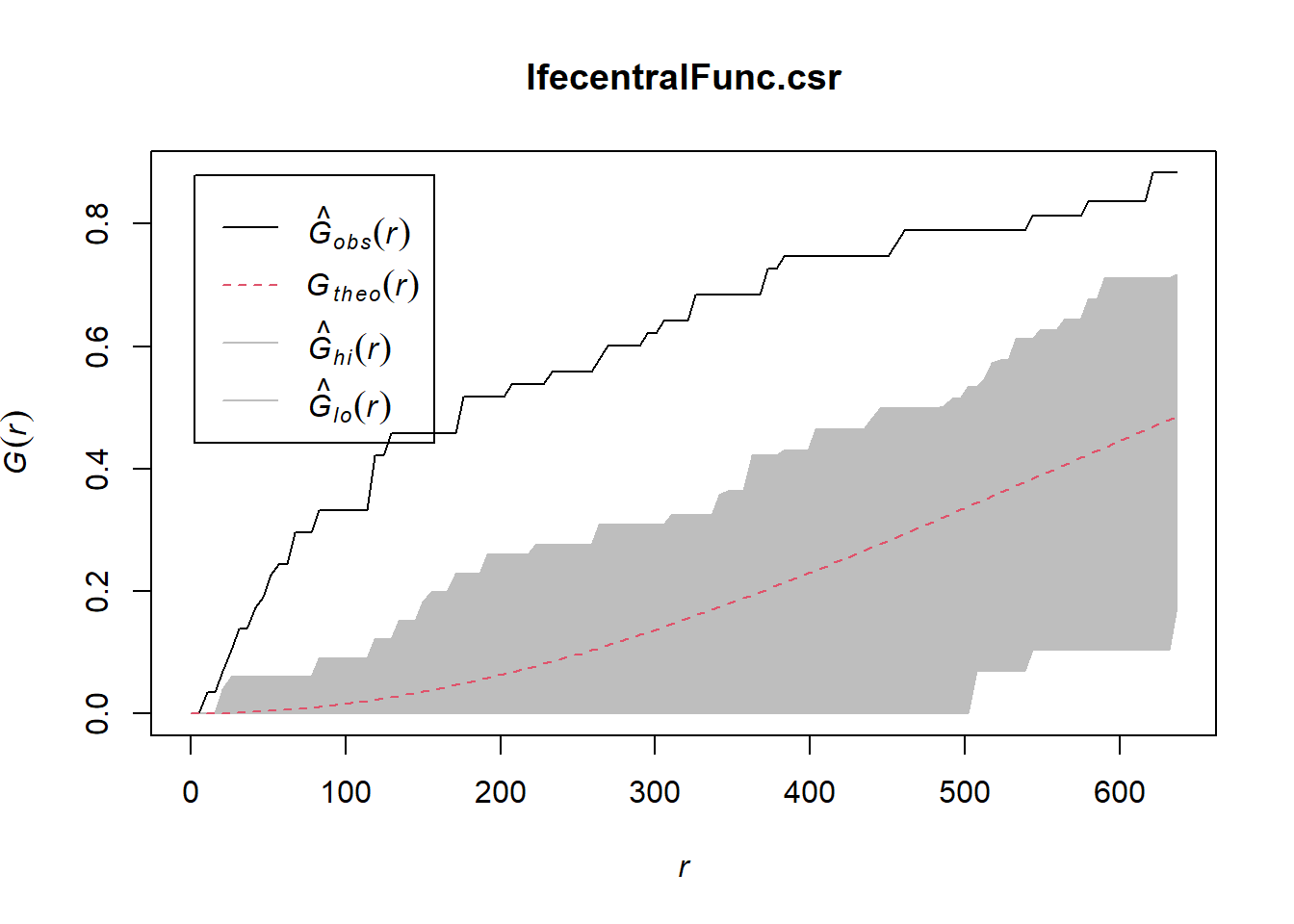
EjigboFuncG = Gest(Ejigboowin_ppp, correction = "border")
plot(EjigboFuncG)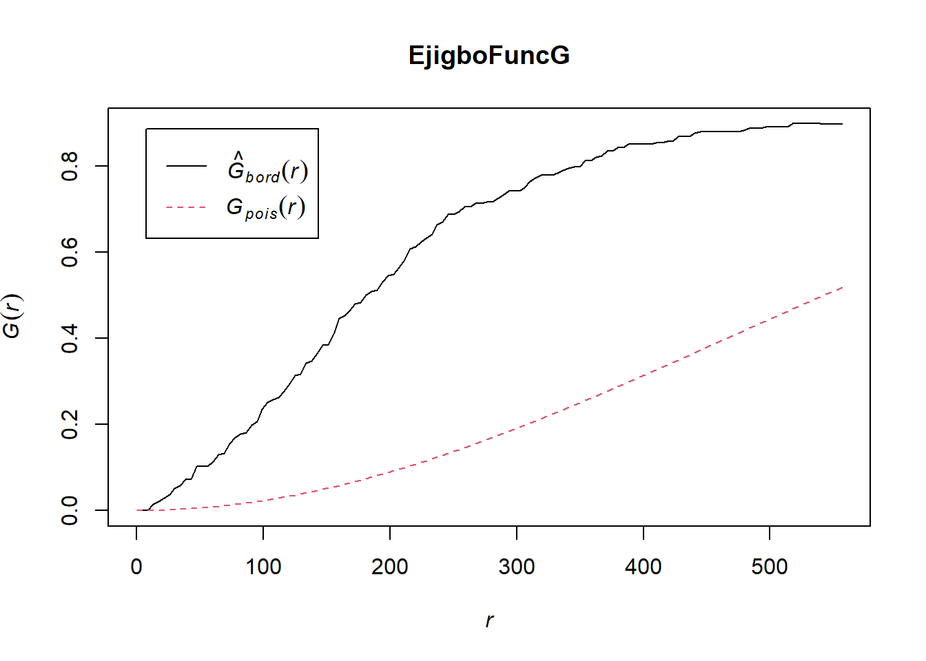
EjigboFunc.csr <- envelope(Ejigboowin_ppp, Gest, nsim=100)Generating 100 simulations of CSR ...
1, 2, 3, 4, 5, 6, 7, 8, 9, 10, 11, 12, 13, 14, 15, 16, 17, 18, 19, 20, 21, 22, 23, 24, 25, 26, 27, 28, 29, 30, 31, 32, 33, 34, 35, 36, 37, 38, 39, 40,
41, 42, 43, 44, 45, 46, 47, 48, 49, 50, 51, 52, 53, 54, 55, 56, 57, 58, 59, 60, 61, 62, 63, 64, 65, 66, 67, 68, 69, 70, 71, 72, 73, 74, 75, 76, 77, 78, 79, 80,
81, 82, 83, 84, 85, 86, 87, 88, 89, 90, 91, 92, 93, 94, 95, 96, 97, 98, 99, 100.
Done.plot(EjigboFunc.csr)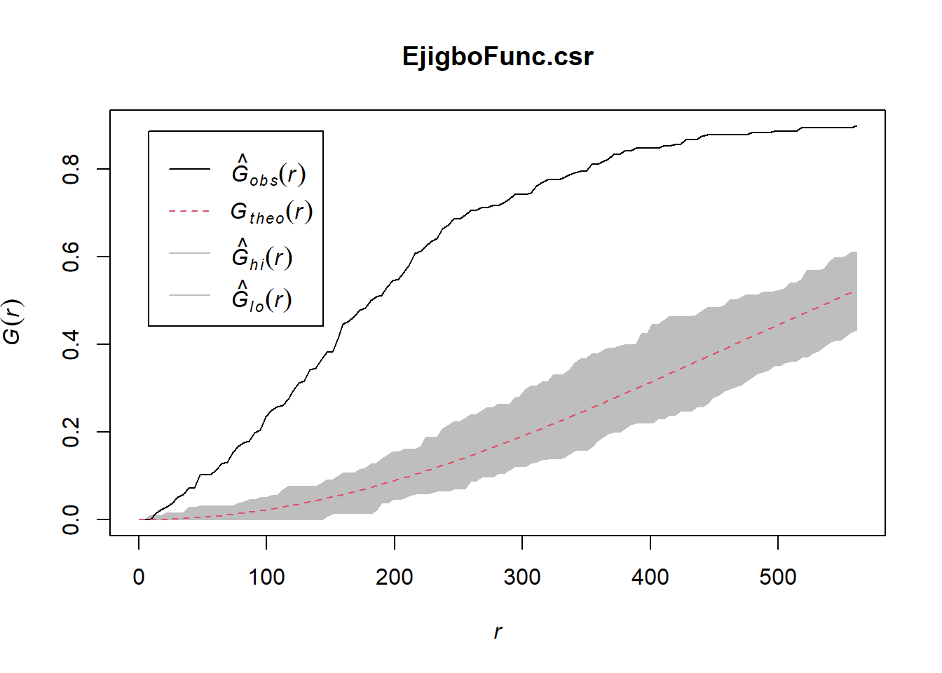
Analysis
In both of the spatial randomness tests for functional waterpoints in the regions of Ife Central, and Ejigbo, we can see that the G(r) is significantly above both G(theo) and the envelope, indicating the functional waterpoints are clustered.Hence we reject the null hypothesis that functional waterpoints are randomly distributed with a 99% confidence
Plotting G function for non-functional waterpoints
EdNorthNonFuncG = Gest(EdeNorthowin_ppp, correction = "border")
plot(EdNorthNonFuncG)
EdNorthNonFunc.csr <- envelope(EdeNorthowin_ppp, Gest, nsim=100)Generating 100 simulations of CSR ...
1, 2, 3, 4, 5, 6, 7, 8, 9, 10, 11, 12, 13, 14, 15, 16, 17, 18, 19, 20, 21, 22, 23, 24, 25, 26, 27, 28, 29, 30, 31, 32, 33, 34, 35, 36, 37, 38, 39, 40,
41, 42, 43, 44, 45, 46, 47, 48, 49, 50, 51, 52, 53, 54, 55, 56, 57, 58, 59, 60, 61, 62, 63, 64, 65, 66, 67, 68, 69, 70, 71, 72, 73, 74, 75, 76, 77, 78, 79, 80,
81, 82, 83, 84, 85, 86, 87, 88, 89, 90, 91, 92, 93, 94, 95, 96, 97, 98, 99, 100.
Done.plot(EdNorthNonFunc.csr)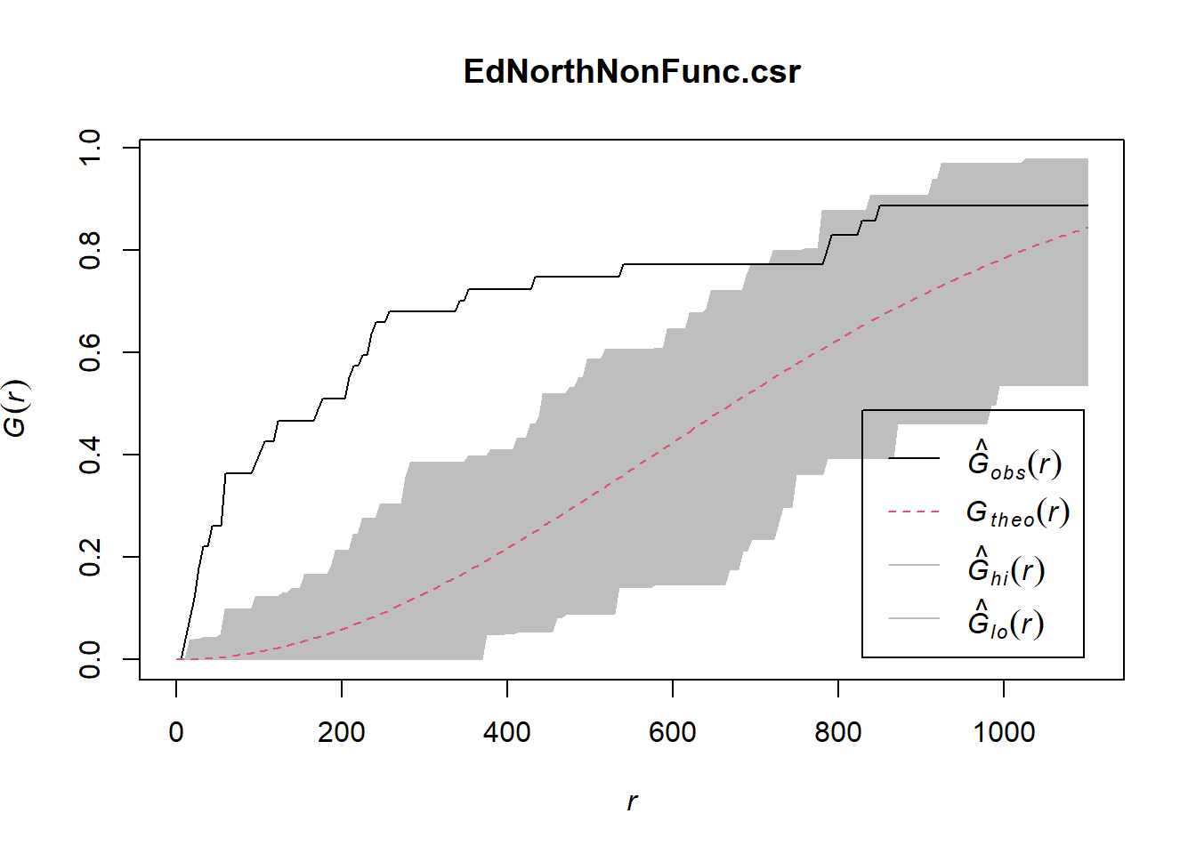
EdSouthNonFuncG = Gest(EdeSouthowin_ppp, correction = "border")
plot(EdSouthNonFuncG)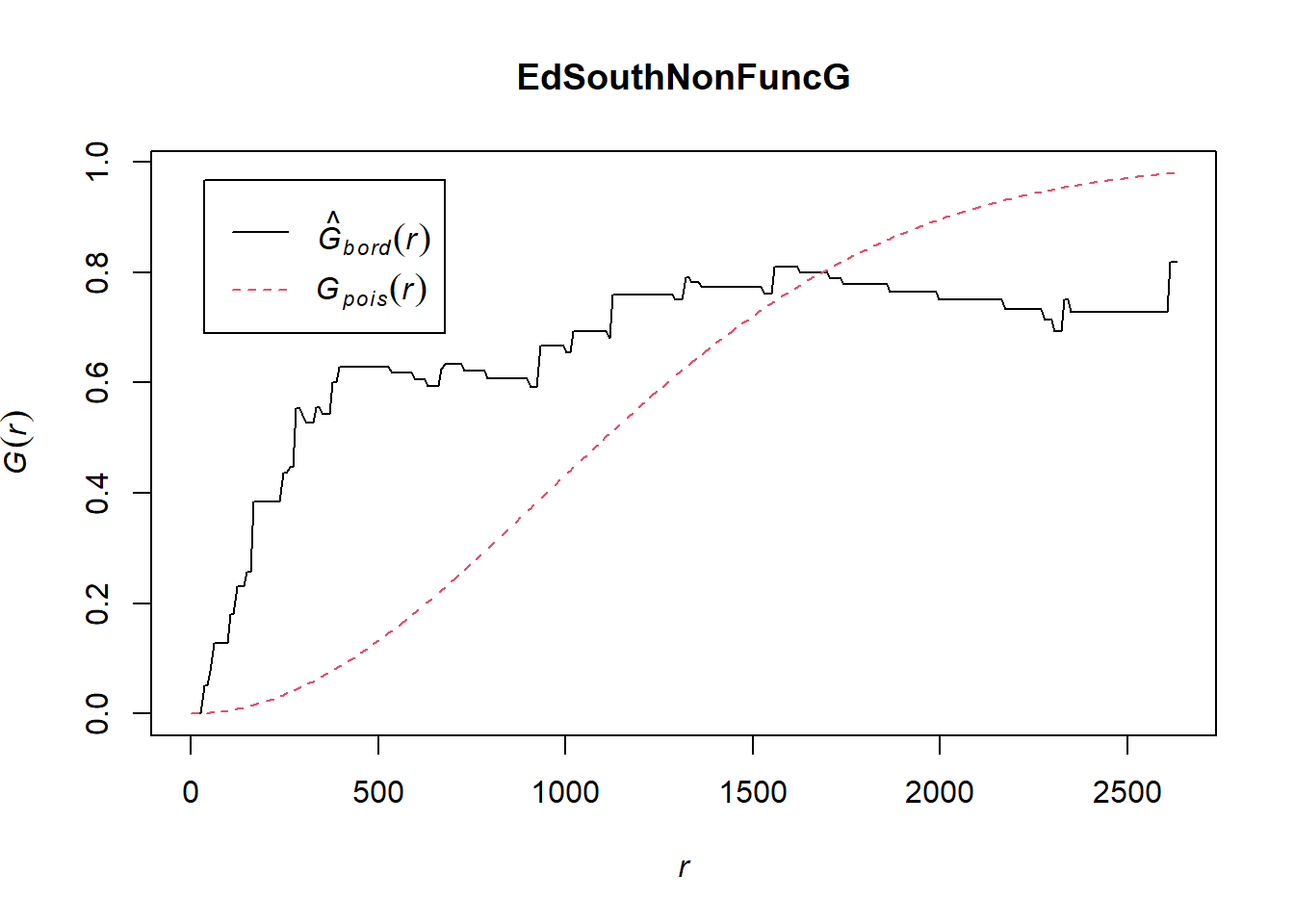
EdSouthNonFunc.csr <- envelope(EdeSouthowin_ppp, Gest, nsim=100)Generating 100 simulations of CSR ...
1, 2, 3, 4, 5, 6, 7, 8, 9, 10, 11, 12, 13, 14, 15, 16, 17, 18, 19, 20, 21, 22, 23, 24, 25, 26, 27, 28, 29, 30, 31, 32, 33, 34, 35, 36, 37, 38, 39, 40,
41, 42, 43, 44, 45, 46, 47, 48, 49, 50, 51, 52, 53, 54, 55, 56, 57, 58, 59, 60, 61, 62, 63, 64, 65, 66, 67, 68, 69, 70, 71, 72, 73, 74, 75, 76, 77, 78, 79, 80,
81, 82, 83, 84, 85, 86, 87, 88, 89, 90, 91, 92, 93, 94, 95, 96, 97, 98, 99, 100.
Done.plot(EdSouthNonFunc.csr)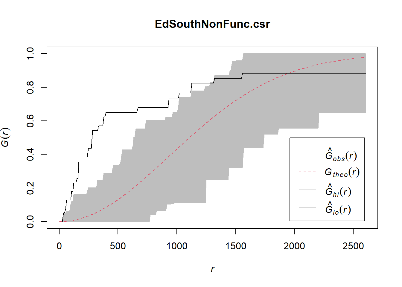
In both of the spatial randomness tests for functional waterpoints in the regions of Ede North, and Ede South, we can see that the G(r) is significantly above both G(theo) and the envelope, indicating the non functional waterpoints are clustered.Hence we reject the null hypothesis that functional waterpoints are randomly distributed with a 99% confidence
Spatial correlation analysis
Local Colocation Quotients (LCLQ)
H0: The Functional Water Points in Osun are not co-located with the Non-Functional Water Points
H1: The Functional Water Points in Osun are co-located with the Non-Functional Water Points
Confidence level : 95%
Significance level (alpha) : 0.05
The null hypothesis will be rejected if p-value < 0.05.
wp_sf_osun_kp <- wp_sf_osun %>%
  filter(`func_status` %in% c("Functional", "Non-Functional"))
functional_points <- wp_sf_osun_kp %>%
filter(`func_status` == "Functional") %>%
dplyr::pull(`func_status`)
nonfunctional_points <- wp_sf_osun_kp %>%
filter(`func_status` == "Non-Functional") %>%
dplyr::pull(`func_status`)Nearest neighbours
nb <- include_self(
  st_knn(st_geometry(wp_sf_osun_kp),6))
Weight matrix
wt <- st_kernel_weights(nb,
                        wp_sf_osun_kp,
                        "gaussian",
                        adaptive = TRUE)
CoLocation Quotient (LCLQ)
LCLQc <- local_colocation(functional_points,
                         nonfunctional_points,
                         nb,
                         wt,
                         39)
LCLQ_waterpoints <- cbind(wp_sf_osun_kp, LCLQc)LCLQ_waterpoints <- LCLQ_waterpoints %>%
mutate(
`p_sim_Non.Functional` = replace(`p_sim_Non.Functional`, `p_sim_Non.Functional` > 0.05, NA),
`Non.Functional` = ifelse(`p_sim_Non.Functional` > 0.05, NA, `Non.Functional`))
LCLQ_waterpoints <- LCLQ_waterpoints %>% mutate(`size` = ifelse(is.na(`Non.Functional`), 1, 5))Analysis
tmap_mode('view')
tm_view(set.zoom.limits=c(9, 15),
        bbox = st_bbox(filter(LCLQ_waterpoints, !is.na(`Non.Functional`)))) +
  tm_shape(NGA) +
  tm_borders() +
  tm_shape(LCLQ_waterpoints) +
  tm_dots(col="Non.Functional",
          palette=c("cyan", "grey"),
          size = "size",
          scale=0.15,
          border.col = "black",
          border.lwd = 0.5,
          alpha=0.5,
          title="LCLQ"
          )
Conclusion
In general the LCLQ value is just slightly less than 1 for statstically significant LCLQ (i.e: p value is < 0.05) . This shows that for a functional waterpoint it is less likely to have a non functional waterpoint in its neighbourhood. This proportion represents the waterpoints proportion across Osun very well.
tmap_mode('plot')