In-class exercise 6

Published

March 25, 2023

Imports

pacman::p_load(sf, sfdep, tmap, tidyverse, knitr)

Importing data

Geospatial

hunan <- st_read(dsn = "data/geospatial", 
                 layer = "Hunan")

Reading layer `Hunan' from data source 
  `C:\Study\Y3\S2\IS415\ELAbishek\IS415-GAA\in-class-exercise\wk6\data\geospatial' 
  using driver `ESRI Shapefile'
Simple feature collection with 88 features and 7 fields
Geometry type: POLYGON
Dimension:     XY
Bounding box:  xmin: 108.7831 ymin: 24.6342 xmax: 114.2544 ymax: 30.12812
Geodetic CRS:  WGS 84

Aspatial

hunan2012 <- read_csv("data/aspatial/Hunan_2012.csv")

Combining data frames using Left join

#Note : To retain geometric column, then left file should be SF and right should be tibbler
hunan_GDPPC <- left_join(hunan,hunan2012)%>%
  select(1:4, 7, 15)

Plotting choropleth map

tmap_mode('plot')
tm_shape(hunan_GDPPC)+
  tm_fill("GDPPC",
          style = "quantile",
          palette = "Blues",
          title = "GDPPC")+
  tm_layout(main.title = "Distribution of GDP per capita by district",
            main.title.position = "center",
            main.title.size = 1.0,
            legend.height = 0.45,
            legend.width = 0.35,
            frame = TRUE) +
  tm_borders(alpha = 0.5) +
  tm_compass(type = "8star", size = 2) +
  tm_scale_bar() +
  tm_grid(alpha = 0.2)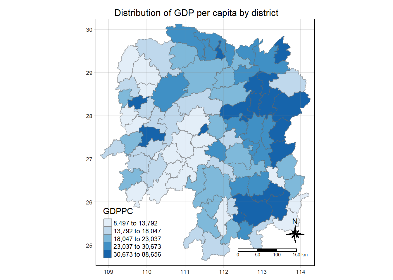

Identify Area neighbours

Contiguity neighbours method (Queen)

cn_queen <- hunan_GDPPC %>%
  mutate(nb = st_contiguity(geometry),
         .before = 1)#Before 1 puts this as the new first column

st_contiguity(hunan_GDPPC, queen = TRUE)

Neighbour list object:
Number of regions: 88 
Number of nonzero links: 448 
Percentage nonzero weights: 5.785124 
Average number of links: 5.090909

Contiguity neighbours method (Rook)

cn_rook <- hunan_GDPPC %>%
  mutate(nb = st_contiguity(geometry),
         queen = FALSE,
         .before = 1)#Before 1 puts this as the new first column

Computing contiguity weights

Contiguity weights (Queen)

wm_q <- hunan_GDPPC %>%
  mutate(nb = st_contiguity(geometry),
         wt = st_weights(nb),
         .before = 1)

Contiguity weights (Rook)

wm_q <- hunan_GDPPC %>%
  mutate(nb = st_contiguity(geometry),
         wt = st_weights(nb),
         queen = FALSE,
         .before = 1)